Graphing and Equations of Two Variables

The Cartesian System

The Cartesian coordinate system is used to visualize points on a graph by showing the points' distances from two axes.

Learning Objectives

Explain how to plot points in the Cartesian plane and what it means to do so

Key Takeaways

Key Points

The Cartesian coordinate system is a 2-dimensional plane with a horizontal axis, known as the $x$ -axis, and a vertical axis, known as the $y$ -axis.
A Cartesian coordinate system specifies each point uniquely in a plane with a pair of numerical coordinates, each of which is the signed distance from the point to one of the two axes.
The numerical coordinates of a point are represented by an ordered pair $(x,y)$ , where the $x$ -coordinate is the point's distance from the $y$ -axis, and the $y$ -coordinate is the distance from the $x$ -axis.
The Cartesian coordinate system is broken into four quadrants, labeled I, II, III, and IV, starting from the upper right hand corner and moving counterclockwise.
The independent variable is found on the $x$ -axis and consists of the input values. The dependent variable is found on the $y$ -axis and consists of the output values.

Key Terms

independent variable: An arbitrary input; on the Cartesian plane, the value of $x$ .
y-axis: The axis on a graph that is usually drawn from bottom to top, with values increasing farther up.
quadrant: One of the four quarters of the Cartesian plane bounded by the $x$ -axis and $y$ -axis.
dependent variable: An arbitrary output; on the Cartesian plane, the value of $y$ .
x-axis: The axis on a graph that is usually drawn from left to right, with values increasing to the right.
ordered pair: A set containing exactly two elements in a fixed order, used to represent a point in a Cartesian coordinate system. Notation: $(x,y)$ .

Named for "the father of analytic geometry," 17th-century French mathematician René Descartes, the Cartesian coordinate system is a 2-dimensional plane with a horizontal axis and a vertical axis. Both axes extend to infinity, and arrows are used to indicate infinite length. The horizontal axis is known as the

x

-axis, and the vertical axis is known as the

y

-axis. The point where the axes intersect is known as the origin. A Cartesian coordinate system is used to graph points. Points are specified uniquely in the Cartesian plane by a pair of numerical coordinates, which are the signed distances from the point to the two axes. Each point can be represented by an ordered pair

(x,y)

, where the

x

-coordinate is the point's distance from the

y

-axis and the

y

-coordinate is the distance from the

x

-axis. The origin where the two axes meet is therefore

(0,0)

. On the

x

-axis, numbers increase toward the right and decrease toward the left; on the

y

-axis, numbers increase going upward and decrease going downward.

A Cartesian coordinate system with the points (0, 0) (the origin, where the x and y axes cross), (2, 3) (2 units to the right and 3 up), (-3, 1) (3 units to the left and 1 up), and (-1.5, -2.5) (1.5 units to the left and 2.5 units down) plotted.

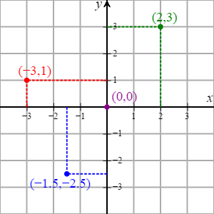Cartesian coordinate system: The Cartesian coordinate system with 4 points plotted, including the origin, at

(0,0)

Plotting Points

To plot the point

(2,3)

, for example, you start at the origin (where the two axes intersect). Then, move three units to the right and two units up. The point

(-3,1)

is found by moving three units to the left of the origin and one unit up. The non-integer coordinates

(-1.5,-2.5)

lie between -1 and -2 on the

x

-axis and between -2 and -3 on the

y

-axis. Therefore, you move one and a half units left and two and a half units down.

Independent and Dependent Variables

A Cartesian plane is particularly useful for plotting a series of points that show a relationship between two variables. For example, there is a relationship between the number of cars a car wash cleans and the money the business makes (its revenue). The revenue, or output, depends upon the number of cars, or input, that they wash. Therefore, the revenue is the dependent variable (

y

), and the number of cars is the independent variable (

x

). The revenue is plotted on the

y

-axis, and the number of cars washed is plotted on the

x

-axis.

Quadrants

The Cartesian coordinate system is broken into four quadrants by the two axes. These quadrants are labeled I, II, III, and IV, starting from the upper right and continuing counter-clockwise, as pictured below.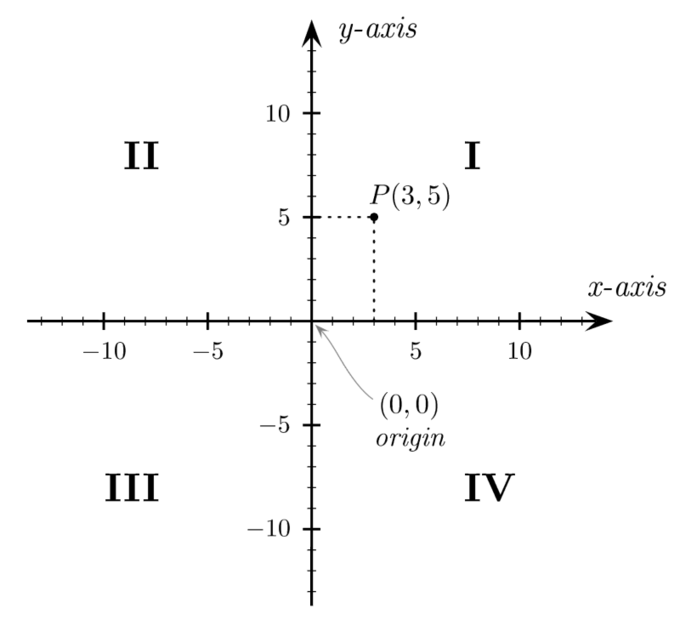

The Cartesian coordinate system with the upper right quadrant labeled I, including the point (3, 5), the upper left quadrant labeled II, the lower left quadrant labeled III, and the lower right quadrant labeled IV.

Cartesian coordinates: The four quadrants of theCartesian coordinate system. The arrows on the axes indicate that they extend infinitely in their respective directions.

Some basic rules about these quadrants can be helpful for quickly plotting points:

Quadrant I: Points have positive $x$ and $y$ coordinates, $(x,y)$ .
Quadrant II: Points have negative $x$ and positive $y$ coordinates, $(-x,y)$ .
Quadrant III: Points have negative $x$ and $y$ coordinates, $(-x,-y)$ .
Quadrant IV: Points have positive $x$ and negative $y$ coordinates, $(x,-y)$ .
Points that have a value of 0 for either coordinate lie on the axes themselves and are not considered to be in any of the quadrants (e.g., $(4,0)$ , $(0,-2)$ ).

Equations in Two Variables

Equations with two unknowns represent a relationship between two variables and have a series of solutions.

Learning Objectives

Explain what an equation in two variables represents

Key Takeaways

Key Points

An equation in two variables has a series of solutions that will satisfy the equation for both variables.
Each solution to an equation in two variables is an ordered pair and can be written in the form $(x, y)$ .

Key Terms

Cartesian coordinates: The coordinates of a point measured from an origin along a horizontal axis from left to right (the $x$ -axis) and along a vertical axis from bottom to top (the $y$ -axis).
ordered pair: A set containing exactly two elements in a fixed order, used to represent a point in a Cartesian coordinate system. Notation: $(x, y)$ .

Equations with two unknowns represent a relationship between two variables. Equations in two variables often express a relationship between the variables

x

and

y

, which correspond to Cartesian coordinates. Equations in two variables have not one solution but a series of solutions that will satisfy the equation for both variables. Each solution is an ordered pair and can be written in the form

(x, y)

Solving Equations in Two Variables

For a given equation in two variables, choosing a value for one variable dictates what the value of the other variable will be. In other words, if a value for one variable is provided, then a solution can be found that satisfies the equation. This is accomplished by substituting the given value in for that variable, and solving for the value of the other.

Example 1

Consider the following equation:

y = 2x

This is an equation in two variables that has an infinite number of solutions. For any

x

-value, the corresponding

y

-value will be twice its value. For example,

(1, 2)

is a solution to the equation. This can be verified by plugging in the

x

- and

y

-values:

(2) = 2(1)

Another solution is

(30, 60)

, because

(60) = 2(30)

. There are thus an infinite number of ordered pairs that satisfy the equation.

Example 2

Now consider the following equation:

y = 2x + 4

Is the point

(3, 10)

a solution to this equation? Note that the ordered pair

(3, 10)

tells us that

x = 3

and

y = 10

. To evaluate whether this is a solution to the equation, substitute these values in for the variables as follows:

(10) = 2(3) + 4

10 = 6 + 4

This is a true statement, so

(3, 10)

is indeed a solution to this equation.

Example 3

Solve the equation

y = 4x - 7

for the value

x=3

. The solution to the given equation would take the form

(x, y)

, and we are given the

x

-value. The

x

-value can be substituted into the equation to find the value of

y

at this point:

y = 4(3) - 7

y = 12 - 7

y = 5

For the given equation,

y = 5

when

x = 3

. Therefore, the solution is

(3, 5)

Example 4

Solve

x + 2y = 8

for

x = 4

. As in the above example, the

x

-value is provided, and we need to find the corresponding

y

-value. We can first rewrite the equation in terms of

y

x + 2y -x = 8 -x

2y = 8 - x

\dfrac{2y}{2} = \dfrac{8-x}{2}

y = \dfrac{8}{2} - \dfrac{x}{2}

y = 4 - \dfrac{1}{2} x

Now substitute

x = 4

into the equation, and solve for

y

y = 4 - \dfrac{1}{2}(4)

y = 4 - 2

y = 2

The solution is

(4, 2)

Graphing Equations

Equations and their relationships can be visualized in many different types of graphs.

Learning Objectives

Practice graphing equations in the Cartesian plane

Key Takeaways

Key Points

Graphs are important tools for visualizing equations.
To graph an equation, choose a value for either $x$ or $y$ , solve for the variable you didn't choose, plot the ordered pair as a point on the Cartesian plane, and repeat, until you have enough points plotted that you can connect them to visualize the graph.

Key Terms

graph: A diagram displaying data; in particular, one showing the relationship between two or more quantities, measurements or numbers.
point: An entity that has a location in space or on a plane, but has no extent.

Now that we know what equations are, how do we go about visualizing them? For an equation with two variables,

x

and

y

, we need a graph with two axes: an

x

-axis and a

y

-axis. We will use the Cartesian plane, in which the

x

-axis is a horizontal line and the

y

-axis is a vertical line. Where the two axes cross is called the origin.

Graphing an Equation in Two Variables

Let's start with the following equation:

y=2x-3

We'll start by choosing a few

x

-values, plugging them into this equation, and solving for the unknown variable

y

. After creating a few

x

and

y

ordered pairs, we will plot them on the Cartesian plane and connect the points. For the three values for

x

, let's choose a negative number, zero, and a positive number so we include points on both sides of the

y

-axis:

If $x=-2$ , then $y=-7$ . We plot the point $(-2,-7)$ .
If $x=0$ , then $y=-3$ . We plot the point $(0,-3)$ .
If $x=2$ , then $y=1$ . We plot the point $(2,1)$ .

Now we can connect the dots to visualize the graph of the equation:

A line with a positive slope, crossing the y-axis at -3 and the x-axis at 1.5.

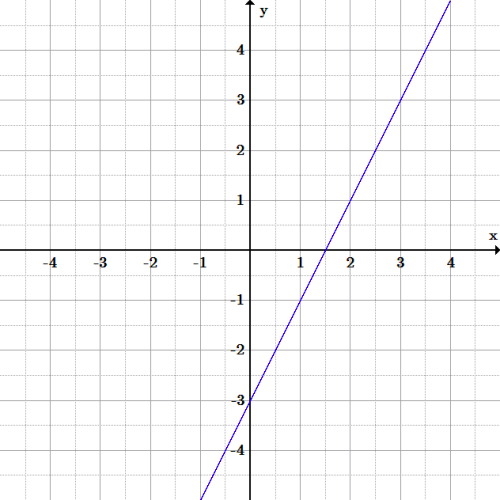Graph of $y=2x-3$ : The equation is the graph of a line through the three points found above. The line continues on to infinity in each direction, since there is an infinite series of ordered pairs of solutions.

Graphing Non-Linear Equations

Example 1

What graph will the following equation make?

x^{2}+y^{2} = 100

Let's figure it out by choosing some points to plot. First, let's try

x=0

\begin{align} (0)^{2}+y^{2} &= 100 \\ y^{2} &= 100 \\ \sqrt{y^{2}}&=\sqrt{100} \\ y &= \pm10 \end{align}

So we plot

(0,10)

and

(0,-10)

. Note that we don't always have to choose values for

x

. For example, let's now try setting

y=0

. Through the same arithmetic as above, we get the ordered pairs

(10,0)

and

(-10,0)

. Plot these as well. We still don't have enough points to really see what's going on, so let's choose some more. Let's try solving for

y

when

x=6

\begin{align} (6)^2+y^2&=100 \\ 36+y^2&=100 \\ 36+y^2-36&=100-36 \\ y^2&=64 \\ y&=\pm 8 \end{align}

So that's two new points:

(6,8)

and

(6,-8)

. We get similar results with

x=-6

, to get

(-6,8)

and

(-6,-8)

. Now you can begin seeing that we're drawing a circle with a radius of 10: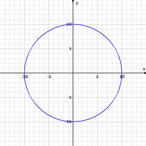

Graph of

x^2+y^2=100

: This is a graph of a circle with radius 10 and center at the origin.

Example 2

Let's try another example. This time let's use the following equation:

y=-x^{2}+9

Again, let's plug in some numbers and begin plotting points. Input values (for the independent variable

x

) from -2 to 2 can be used to obtain output values (the dependent variable

y

) from 5 to 9. Connect these points with the best curve you can, and you'll discover you've drawn a parabola.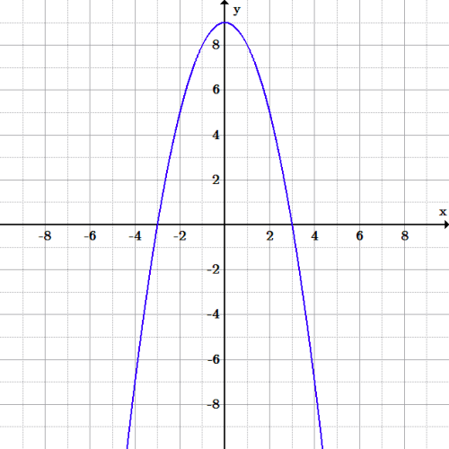

A parabola opening down to make a hill shape, with the vertex (top) at (0, 9), and crossing the x-axis at 3 and -3, continuing down in both directions.

Graph of

y=-x^2+9

: This graph is of a parabola (a U-shaped open curve symmetric about a line). Parabolas can open up or down, right or left; they also have a maximum or minimum value.

Graphs of Equations as Graphs of Solutions

A solution to an equation can be plotted on graphs to better visualize how the equation, or function, behaves.

Learning Objectives

Recognize that graphing an equation involves graphing solutions to it

Key Takeaways

Key Points

To solve an equation is to find what values (numbers, functions, sets, etc.) fulfill a condition stated in the form of an equation.
Once an equation has been graphed, solutions to any particular $x$ or $y$ value can be readily found by simply looking at the graph.
To solve for a variable of an equation, you must use algebraic manipulations to get the variable by itself on one side of the equation (typically the left).

Key Terms

equation: An assertion that two expressions are equivalent (e.g., $x=5$ ).
graph: A diagram displaying data, generally representing the relationship between two or more quantities.
expression: An arrangement of symbols denoting values, operations performed on them, and grouping symbols (e.g., $(2x+4)$ ).

In mathematics, to solve an equation is to find what values (numbers, functions, sets, etc.) fulfill a condition stated in the form of an equation (two expressions related by equality). Each of the expressions contain one or more unknowns. What is the graphical difference between equations with one variable and equations with two variables?

Graphs of Linear Equations with One Variable

A linear equation in one variable can be written in the form

ax+b=0,

where

a

and

b

are real numbers and

a\neq 0

. In an equation where

x

is a real number, the graph is the collection of all ordered pairs with any value of

y

paired with that real number for

x

. For example, to graph the equation

x-1=0,

a few of the ordered pairs would include:

$(1,-3)$
$(1,-2)$
$(1,-1)$
$(1,0)$
$(1,1)$
$(1,2)$
$(1,3)$

These can also be found by solving the equation of the graph for

x

, which yields

x = 1

. This means that the

y

-values of the points don't matter as long as their

x

-values are 1. The graph is therefore a vertical line through those points, since all points have the same

x

-value. The same is true for an equation written as

ay+b=0

, or

y=-4

, for example. The graph would be a horizontal line through points that all have

y

-values of -4. Therefore, when the equation is

y=C,

where

C

is a constant real number, the graph is a horizontal line. Similarly, if the equation is

x=C,

then the graph is a vertical line.

Graphs of Equations with Two Variables

The graph of a cubic polynomial has an equation like

y=x^3-9x

. Its equation has two variables,

x

and

y

, and the equation is solved for

y

. Plot specific points by substituting chosen

x

-values into the equation, and solve for the corresponding

y

value, and then graph. Let's choose values for

x

from -2 to 2. When

x=-2

, we have:

y=(-2)^3-9(-2)=(-8)+18=10

Therefore,

(-2,10)

is a point on this curve (i.e., the graph of the equation). After substituting the rest of the values, the following ordered pairs are found:

$(-1,8)$
$(0,0)$
$(1,-8)$
$(2,-10)$

After graphing the ordered pairs and connecting the points, we see that the set of (infinite) points follows this pattern:

The cubic polynomial is negative for x-values less than negative 3, then takes the shape of a hill from x = -3 to x = 0 with a peak of around 10 between x = -2 and x = -1. From x = 0 to x = 3 it has a valley shape with the lowest point of about -10 between x = 1 and x = 2, crossing the x-axis at x=3, then continuing up infinitely for x-values greater than 3.

Graph of

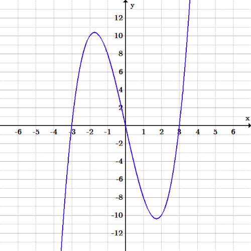y=x^3-9x

: Since the exponent of

x

is a 3, it means that this equation is a 3rd-degree polynomial, called a cubic polynomial.

Graphing Inequalities

The solutions to inequalities can be graphed by drawing a boundary line to divide the coordinate plane in two and shading in one of those parts.

Learning Objectives

Practice graphing inequalities by shading in the correct section of the plane

Key Takeaways

Key Points

All solutions to a given inequality are located in one half-plane and can be graphed.
To graph an inequality, first treat it as a linear equation and graph the corresponding line. Then, shade the correct half-plane to represent all the possible solutions to the inequality.
If an inequality uses a $\leq$ or $\geq$ symbol, the boundary line should be drawn solid, meaning that solutions include points on the line itself.
If an inequality uses a $<$ or $>$ symbol, the boundary line should be drawn dotted, meaning that solutions do not include any points on the line.

Key Terms

half-plane: One of the two parts of the coordinate plane created when a line is drawn.
boundary line: The straight line in the graph of an inequality that defines the half-plane containing the solutions to the inequality.

In our study of linear equations in two variables, we observed that all the solutions to an equation—and only those solutions— were located on the graph of that equation. We now wish to determine the location of the solutions to linear inequalities in two variables. Linear inequalities in two variables have one of the following forms:

$ac + by < c$
$ac + by \leq c$
$ac + by > c$
$ac + by \geq c$

Recall that for a linear equation in two variables, ordered pairs that produce true statements when substituted into the equation are called "solutions" to that equation. We can make a similar statement regarding inequalities in two variables. We say that an inequality in two variables has a solution when a pair of values has been found such that substituting these values into the inequality results in a true statement. As with equations, solutions to linear inequalities have particular locations in the coordinate plane. For a linear equality in two variables, all solutions are located in one entire half-plane. A straight line drawn through the plane divides the plane into two half-planes, as shown in the diagram below. The straight line shown is called a boundary line.

Slanted boundary line dividing the Cartesian plane into two half planes.

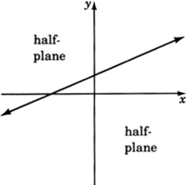Half-planes: The boundary line shown above divides the coordinate plane into two half-planes.

For example, consider the following inequality:

2x + 3y \leq 6

The graph below demonstrates all solutions to this inequality, which fall on the boundary line and in the shaded half-plane.

The Cartesian plane with the line 2x+3y = 6 graphed, having a negative slope and passing through the points (0, 2) and (3, 0). The area below the line is shaded, indicating that all points in the half-plane below the line (for example, (1, -1)) are solutions, and that all points in the half-plane above the line (for example, (2, 5)) are not.

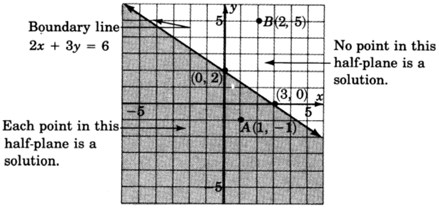Graph of $2x + 3y \leq 6$ : All points lying on the boundary line and in the shaded half-plane are solutions to this inequality.

Now consider the following inequality:

y > 2

The graph below shows the solutions to this inequality: the shaded area above the boundary line. Note that because the inequality uses the

>

symbol, rather than the

\geq

symbol, the inequality is strict: points on the boundary line are not solutions, so the line is drawn dotted.

A Cartesian plane with a horizontal dotted line through (0, 2).

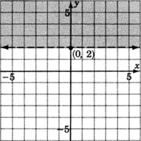Graph of $y > 2$ : All points in the shaded half-plane above the line are solutions to this inequality.

The method of graphing linear inequalities in two variables is as follows.

First, consider the inequality as an equation (i.e., replace the inequality sign with an equals sign) and graph that equation. This is called the boundary line. Note:

If the inequality is $\leq$ or $\geq$ , draw the boundary line solid. This means that points on the line are solutions and are part of the graph.
If the inequality is $<$ or $>$ , draw the boundary line dotted. This means that points on the line are not solutions and are not part of the graph.

Determine which half-plane to shade by choosing a test point.

If, when substituted, the test point yields a true statement, shade the half-plane containing it.
If, when substituted, the test point yields a false statement, shade the half-plane on the opposite side of the boundary line.

Example 1

Graph the following inequality:

3x - 2y \geq -4

First, we need to graph the boundary line. To do so, consider the inequality as an equation:

3x−2y=−4

Recall that, in order to graph an equation, we can substitute a value for one variable and solve for the other. The resulting ordered pair will be one solution to the equation. So, let's substitute

x = 0

to find one solution:

\begin{align} 3(0) - 2y &= -4 \\ - 2y &= -4 \\ \dfrac{-2y}{-2} &= \dfrac{-4}{-2} \\ y &= 2 \end{align}

Now let's substitute

y=0

to find another solution:

\begin{align} 3x - 2(0) &= - 4 \\ 3x &= -4 \\ \dfrac{3x}{3} &= \dfrac{-4}{3} \\ x &= - \dfrac{4}{3} \end{align}

Now we can graph the two known solutions,

(0, 2)

and

(-\frac{4}{3}, 0)

. The inequality is

\geq

, so we know we need to draw the line solid. This gives the boundary line below: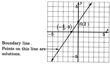

The boundary line through the two given points is drawn; it has positive slope. Points on the boundary line are solutions.

Graph of boundary line for $3x - 2y \geq -4$ : Graph of the boundary line, drawn using two ordered-pair solutions.

Next, choose a test point to figure out which half-plane we need to shade in. The easiest test point is

(0, 0)

. Let's substitute

(0, 0)

into the original inequality:

\begin{align} 3(0) - 2(0) &\geq -4 \\ 0 &\geq -4 \end{align}

This a true statement, so shade in the half-plane containing

(0, 0).

The region below the boundary line, including the test point (0, 0), is shaded; points in this region are solutions. The area above the boundary line is not shaded, indicating that points in this region are not solutions.

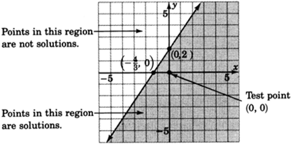Graph of $3x - 2y \geq -4$ : Graph showing all possible solutions of the given inequality. The solutions lie in the shaded region, including the boundary line.

Licenses & Attributions

CC licensed content, Shared previously

Curation and Revision. Authored by: Boundless.com. License: Public Domain: No Known Copyright.

CC licensed content, Specific attribution

Intermediate Algebra/The Coordinate (Cartesian) Plane. Provided by: Wikibooks Located at: https://en.wikibooks.org/wiki/Intermediate_Algebra/The_Coordinate_(Cartesian)_Plane. License: CC BY-SA: Attribution-ShareAlike.
Dependent and independent variables. Provided by: Wikipedia License: CC BY: Attribution.
Cartesian-coordinate-system. Provided by: Wikimedia License: Public Domain: No Known Copyright.
2D Cartesian Coordinates. Provided by: Wikipedia License: CC BY-SA: Attribution-ShareAlike.
Algebra/The Coordinate (Cartesian) Plane. Provided by: Wikibooks License: CC BY-SA: Attribution-ShareAlike.
quadrant. Provided by: Wiktionary License: CC BY-SA: Attribution-ShareAlike.
Boundless. Provided by: Boundless Learning License: CC BY-SA: Attribution-ShareAlike.
y-axis. Provided by: Wiktionary License: CC BY-SA: Attribution-ShareAlike.
x-axis. Provided by: Wiktionary License: CC BY-SA: Attribution-ShareAlike.
Cartesian-coordinate-system. Provided by: Wikimedia License: Public Domain: No Known Copyright.
Cartesian Coordinate System. Provided by: Wikipedia License: CC BY-SA: Attribution-ShareAlike.
Cartesian coordinate. Provided by: Wikipedia Located at: https://en.wiktionary.org/wiki/Cartesian_coordinate. License: CC BY-SA: Attribution-ShareAlike.
Equation. Provided by: Wikipedia License: CC BY-SA: Attribution-ShareAlike.
Cartesian coordinate system. Provided by: Wikipedia License: CC BY-SA: Attribution-ShareAlike.
Cartesian-coordinate-system. Provided by: Wikimedia License: Public Domain: No Known Copyright.
Cartesian Coordinate System. Provided by: Wikipedia License: CC BY-SA: Attribution-ShareAlike.
Algebra/Function Graphing. Provided by: Wikibooks License: CC BY-SA: Attribution-ShareAlike.
Algebra/Equations. Provided by: Wikibooks License: CC BY-SA: Attribution-ShareAlike.
point. Provided by: Wikipedia License: CC BY-SA: Attribution-ShareAlike.
graph. Provided by: Wiktionary License: CC BY-SA: Attribution-ShareAlike.
Graph of a function. Provided by: Wikipedia License: CC BY-SA: Attribution-ShareAlike.
Cartesian-coordinate-system. Provided by: Wikimedia License: Public Domain: No Known Copyright.
Cartesian Coordinate System. Provided by: Wikipedia License: CC BY-SA: Attribution-ShareAlike.
Original figure by Julien Coyne. Licensed CC BY-SA 4.0. Provided by: Julien Coyne License: CC BY-SA: Attribution-ShareAlike.
Original figure by Julien Coyne. Licensed CC BY-SA 4.0. Provided by: Julien Coyne License: CC BY-SA: Attribution-ShareAlike.
Original figure by Julien Coyne. Licensed CC BY-SA 4.0. Provided by: Julien Coyne License: CC BY-SA: Attribution-ShareAlike.
Algebra/Equations. Provided by: Wikibooks License: CC BY-SA: Attribution-ShareAlike.
Graph of a function. Provided by: Wikipedia License: CC BY-SA: Attribution-ShareAlike.
Equations. Provided by: Wikipedia License: CC BY-SA: Attribution-ShareAlike.
Algebra/Function Graphing. Provided by: Wikibooks License: CC BY-SA: Attribution-ShareAlike.
Algebra/Solving Equations. Provided by: Wikibooks License: CC BY-SA: Attribution-ShareAlike.
Equation solving. Provided by: Wikipedia License: CC BY-SA: Attribution-ShareAlike.
expression. Provided by: Wiktionary License: CC BY-SA: Attribution-ShareAlike.
equation. Provided by: Wiktionary License: CC BY-SA: Attribution-ShareAlike.
graph. Provided by: Wiktionary License: CC BY-SA: Attribution-ShareAlike.
Linear Equations in One Variable. Provided by: Openstax Located at: https://openstax.org/books/college-algebra/pages/2-2-linear-equations-in-one-variable. License: CC BY-SA: Attribution-ShareAlike.
Cartesian-coordinate-system. Provided by: Wikimedia License: Public Domain: No Known Copyright.
Cartesian Coordinate System. Provided by: Wikipedia License: CC BY-SA: Attribution-ShareAlike.
Original figure by Julien Coyne. Licensed CC BY-SA 4.0. Provided by: Julien Coyne License: CC BY-SA: Attribution-ShareAlike.
Original figure by Julien Coyne. Licensed CC BY-SA 4.0. Provided by: Julien Coyne License: CC BY-SA: Attribution-ShareAlike.
Original figure by Julien Coyne. Licensed CC BY-SA 4.0. Provided by: Julien Coyne License: CC BY-SA: Attribution-ShareAlike.
Original figure by Julien Coyne. Licensed CC BY-SA 4.0. Provided by: Julien Coyne License: CC BY-SA: Attribution-ShareAlike.
Graphing Linear Equations and Inequalities: Graphing Linear Inequalities in Two Variables. Provided by: Wade Ellis and Denny Burzynski, OpenStax CNX. Jun 1, 2009 Located at: https://cnx.org/contents/82f983c0-84ab-49a3-a86e-9004eb8d1fcb@4. License: CC BY: Attribution.
Cartesian-coordinate-system. Provided by: Wikimedia Located at: https://commons.wikimedia.org/wiki/File:Cartesian-coordinate-system.svg. License: Public Domain: No Known Copyright.
Cartesian Coordinate System. Provided by: Wikipedia License: CC BY-SA: Attribution-ShareAlike.
Original figure by Julien Coyne. Licensed CC BY-SA 4.0. Provided by: Julien Coyne License: CC BY-SA: Attribution-ShareAlike.
Original figure by Julien Coyne. Licensed CC BY-SA 4.0. Provided by: Julien Coyne License: CC BY-SA: Attribution-ShareAlike.
Original figure by Julien Coyne. Licensed CC BY-SA 4.0. Provided by: Julien Coyne License: CC BY-SA: Attribution-ShareAlike.
Original figure by Julien Coyne. Licensed CC BY-SA 4.0. Provided by: Julien Coyne License: CC BY-SA: Attribution-ShareAlike.
Graphing Linear Equations and Inequalities: Graphing Linear Inequalities in Two Variables. . Provided by: Wade Ellis and Denny Burzynski, OpenStax CNX. Jun 1, 2009 Located at: https://cnx.org/contents/82f983c0-84ab-49a3-a86e-9004eb8d1fcb@4. License: CC BY: Attribution.
Graphing Linear Equations and Inequalities: Graphing Linear Inequalities in Two Variables. Provided by: Wade EllisDenny Burzynski, OpenStax CNX. Jun 1, 2009 License: CC BY: Attribution.
Graphing Linear Equations and Inequalities: Graphing Linear Inequalities in Two Variables. . Provided by: Wade Ellis and Denny Burzynski, OpenStax CNX. Jun 1, 2009 Located at: https://cnx.org/contents/82f983c0-84ab-49a3-a86e-9004eb8d1fcb@4. License: CC BY: Attribution.
Graphing Linear Equations and Inequalities: Graphing Linear Inequalities in Two Variables. Provided by: Wade Ellis and Denny Burzynski, Graphing Linear Equations and Inequalities: Graphing Linear Inequalities in Two Variables. OpenStax CNX. Jun 1, 2009 License: CC BY: Attribution.
Graphing Linear Equations and Inequalities: Graphing Linear Inequalities in Two Variables. Provided by: Wade Ellis and Denny Burzynski, OpenStax CNX. Jun 1, 2009 Located at: https://cnx.org/contents/82f983c0-84ab-49a3-a86e-9004eb8d1fcb@4. License: CC BY: Attribution.

Study Guides > Boundless Algebra

Graphing and Equations of Two Variables

The Cartesian System

Learning Objectives

Key Takeaways

Key Points

Key Terms

Plotting Points

Independent and Dependent Variables

Quadrants

Equations in Two Variables

Learning Objectives

Key Takeaways

Key Points

Key Terms

Solving Equations in Two Variables

Example 1

Example 2

Example 3

Example 4

Graphing Equations

Learning Objectives

Key Takeaways

Key Points

Key Terms

Graphing an Equation in Two Variables

Example 1

Example 2

Graphs of Equations as Graphs of Solutions

Learning Objectives

Key Takeaways

Key Points

Key Terms

Graphs of Linear Equations with One Variable

Graphs of Equations with Two Variables

Graphing Inequalities

Learning Objectives

Key Takeaways

Key Points

Key Terms

Example 1

Licenses & Attributions

CC licensed content, Shared previously

CC licensed content, Specific attribution