Second-Order Linear Equations
Second-Order Linear Equations
A second-order linear differential equation has the form [latex]\frac{d^2 y}{dt^2} + A_1(t)\frac{dy}{dt} + A_2(t)y = f(t)[/latex], where [latex]A_1(t)[/latex], [latex]A_2(t)[/latex], and [latex]f(t)[/latex] are continuous functions.Learning Objectives
Distinguish homogeneous and nonhomogeneous second-order linear differential equationsKey Takeaways
Key Points
- Linear differential equations are of the form [latex]L [y(t)] = f(t)[/latex], where [latex]L_n(y) \equiv \frac{d^n y}{dt^n} + A_1(t)\frac{d^{n-1}y}{dt^{n-1}} + \cdots + A_{n-1}(t)\frac{dy}{dt} + A_n(t)y[/latex].
- When [latex]f(t)=0[/latex], the equations are called homogeneous linear differential equations. (Otherwise, the equations are called nonhomogeneous equations).
- Linear differential equations are differential equations that have solutions which can be added together to form other solutions.
Key Terms
- linear: having the form of a line; straight
- differential equation: an equation involving the derivatives of a function
Second-Order Linear Differential Equations
A second-order linear differential equation has the form: [latex-display]\displaystyle{\frac{d^2 y}{dt^2} + A_1(t)\frac{dy}{dt} + A_2(t)y = f(t)}[/latex-display] where [latex]A_1(t)[/latex], [latex]A_2(t)[/latex], and [latex]f(t)[/latex] are continuous functions. When [latex]f(t)=0[/latex], the equations are called homogeneous second-order linear differential equations. (Otherwise, the equations are called nonhomogeneous equations.)
Simple Pendulum: A simple pendulum, under the conditions of no damping and small amplitude, is described by a equation of motion which is a second-order linear differential equation.
Nonhomogeneous Linear Equations
Nonhomogeneous second-order linear equation are of the the form: [latex]\frac{d^2 y}{dt^2} + A_1(t)\frac{dy}{dt} + A_2(t)y = f(t)[/latex], where [latex]f(t)[/latex] is nonzero.Learning Objectives
Identify when a second-order linear differential equation can be solved analyticallyKey Takeaways
Key Points
- Examples of homogeneous or nonhomogeneous second-order linear differential equation can be found in many different disciplines such as physics, economics, and engineering.
- In simple cases, for example, where the coefficients [latex]A_1(t)[/latex] and [latex]A_2(t)[/latex] are constants, the equation can be analytically solved. In general, the solution of the differential equation can only be obtained numerically.
- Linear differential equations are differential equations that have solutions which can be added together to form other solutions.
Key Terms
- linearity: a relationship between several quantities which can be considered proportional and expressed in terms of linear algebra; any mathematical property of a relationship, operation, or function that is analogous to such proportionality, satisfying additivity and homogeneity
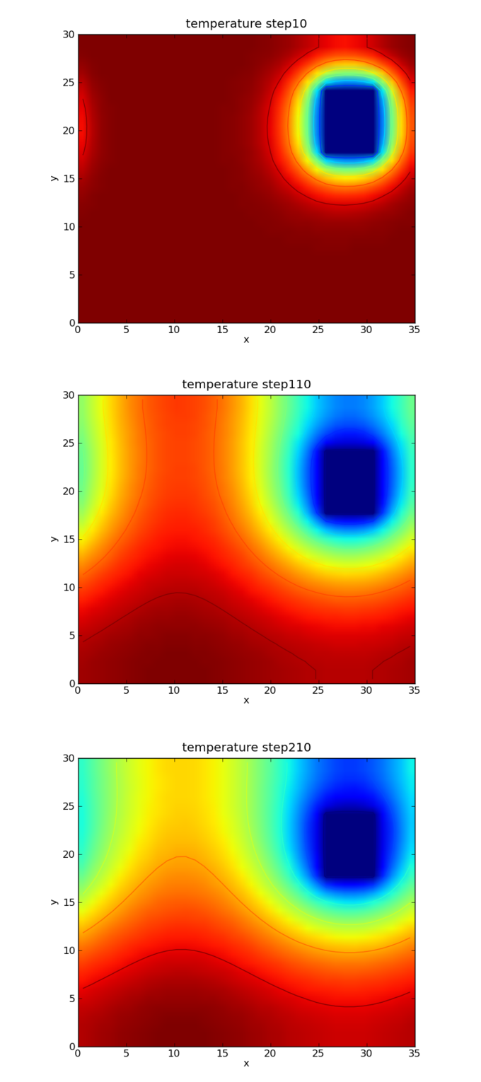
Heat Transfer: Phenomena such as heat transfer can be described using nonhomogeneous second-order linear differential equations.
Linearity
Linear differential equations are differential equations that have solutions which can be added together to form other solutions. If [latex]y_1(t)[/latex] and [latex]y_2(t)[/latex] are both solutions of the second-order linear differential equation provided above and replicated here: [latex-display]\displaystyle{\frac{d^2 y}{dt^2} + A_1(t)\frac{dy}{dt} + A_2(t)y = f(t)}[/latex-display] then any arbitrary linear combination of [latex]y_1(t)[/latex] and [latex]y_2(t)[/latex] —that is, [latex]y(x) = c_1y_1(t) + c_2 y_2(t)[/latex] for constants [latex]c_1[/latex] and [latex]c_2[/latex]—is also a solution of that differential equation. This can be confirmed by substituting [latex]y(x) = c_1y_1(t) + c_2 y_2(t)[/latex] into the equation and using the fact that both [latex]y_1(t)[/latex] and [latex]y_2(t)[/latex] are solutions of the equation.Applications of Second-Order Differential Equations
A second-order linear differential equation can be commonly found in physics, economics, and engineering.Learning Objectives
Identify problems that require solution of nonhomogeneous and homogeneous second-order linear differential equationsKey Takeaways
Key Points
- An ideal spring with a spring constant [latex]k[/latex] is described by the simple harmonic oscillation, whose equation of motion is given in the form of a homogeneous second-order linear differential equation: [latex]m \frac{\mathrm{d}^2x}{\mathrm{d}t^2} + k x = 0[/latex].
- Adding the damping term in the equation of motion, the equation of motion is given as [latex]\frac{\mathrm{d}^2x}{\mathrm{d}t^2} + 2\zeta\omega_0\frac{\mathrm{d}x}{\mathrm{d}t} + \omega_0^{\,2} x = 0[/latex].
- Adding the external force term to the damped harmonic oscillator, we get an nonhomogeneous second-order linear differential equation:[latex]\frac{\mathrm{d}^2x}{\mathrm{d}t^2} + 2\zeta\omega_0\frac{\mathrm{d}x}{\mathrm{d}t} + \omega_0^2 x = \frac{F(t)}{m}[/latex].
Key Terms
- damping: the reduction in the magnitude of oscillations by the dissipation of energy
- harmonic oscillator: a system which, when displaced from its equilibrium position, experiences a restoring force proportional to the displacement according to Hooke's law, where [latex]k[/latex] is a positive constant
Harmonic oscillator
In classical mechanics, a harmonic oscillator is a system that, when displaced from its equilibrium position, experiences a restoring force, [latex]F[/latex], proportional to the displacement, [latex]x[/latex]: [latex]\vec F = -k \vec x \,[/latex], where [latex]k[/latex] is a positive constant. The system under consideration could be an object attached to a spring, a pendulum, etc. Electronic circuits such as RLC circuits are also described by similar equations.Simple harmonic oscillation
If [latex]F[/latex] is the only force acting on the system, the system is called a simple harmonic oscillator, and it undergoes simple harmonic motion: sinusoidal oscillations about the equilibrium point, with a constant amplitude and a constant frequency. The equation of motion is given as: [latex-display]\displaystyle{F = m a = m \frac{\mathrm{d}^2x}{\mathrm{d}t^2} = -k x}[/latex-display] Therefore, we end up with a homogeneous second-order linear differential equation: [latex-display]\displaystyle{m \frac{\mathrm{d}^2x}{\mathrm{d}t^2} + k x = 0}[/latex-display] Note that the function [latex]x(t) = A\cos\left( \omega_0 t+\phi\right)[/latex] satisfies the equation where [latex]\omega_0 = \sqrt{\frac{k}{m}} = \frac{2\pi}{T}[/latex]. [latex]\omega_0[/latex] is called angular velocity, and the constants [latex]A[/latex] and [latex]\phi[/latex] are determined from initial conditions of the motion.Damped harmonic oscillator
In real oscillators, friction (or damping) slows the motion of the system. In many vibrating systems the frictional force [latex]Ff[/latex] can be modeled as being proportional to the velocity v of the object: [latex]Ff = −cv[/latex], where [latex]c[/latex] is called the viscous damping coefficient. Including this additional term, the equation of motion is given as: [latex-display]\displaystyle{\frac{\mathrm{d}^2x}{\mathrm{d}t^2} + 2\zeta\omega_0\frac{\mathrm{d}x}{\mathrm{d}t} + \omega_0^{\,2} x = 0}[/latex-display] where [latex]\zeta = \frac{c}{2 \sqrt{mk}}[/latex] is called the "damping ratio."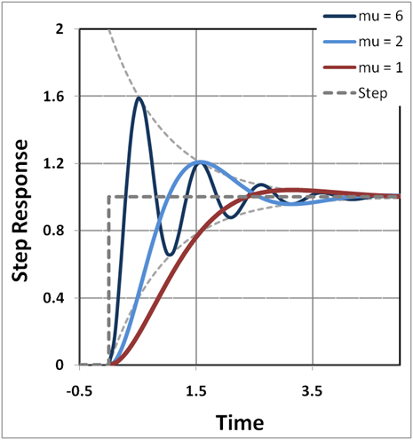
Damped Harmonic Oscillators: A solution of damped harmonic oscillator. Curves in different colors show various responses depending on the damping ratio.
Series Solutions
The power series method is used to seek a power series solution to certain differential equations.Learning Objectives
Identify the steps and describe the application of the power series methodKey Takeaways
Key Points
- The power series method calls for the construction of a power series solution [latex]f=\sum_{k=0}^\infty A_kz^k[/latex] for a linear differential equation [latex]f''+{a_1(z)\over a_2(z)}f'+{a_0(z)\over a_2(z)}f=0[/latex].
- The method assumes a power series with unknown coefficients, then substitutes that solution into the differential equation to find a recurrence relation for the coefficients.
- Hermit differential equation [latex]f''-2zf'+\lambda f=0;\;\lambda=1[/latex] has the following power series solution: [latex]f=A_0 \left(1+{-1\over 2}x^2+{-1 \over 8}x^4+{-7 \over 240}x^6+\cdots\right) + A_1\left(x+{1\over 6}x^3+{1 \over 24}x^5+{1 \over 112}x^7+\cdots\right)[/latex].
Key Terms
- recurrence relation: an equation that recursively defines a sequence; each term of the sequence is defined as a function of the preceding terms
- analytic functions: a function that is locally given by a convergent power series
Maclaurin Power Series of an Exponential Function: The exponential function (in blue), and the sum of the first [latex]n+1[/latex] terms of its Maclaurin power series (in red). Using power series, a linear differential equation of a general form may be solved.
Method
Consider the second-order linear differential equation: [latex-display]a_2(z)f''(z)+a_1(z)f'(z)+a_0(z)f(z)=0[/latex-display] Suppose [latex]a_2[/latex] is nonzero for all [latex]z[/latex]. Then we can divide throughout to obtain: [latex-display]\displaystyle{f''+{a_1(z)\over a_2(z)}f'+{a_0(z)\over a_2(z)}f=0}[/latex-display] Suppose further that [latex]\frac{a_1}{a_2}[/latex] and [latex]\frac{a_1}{a_2}[/latex] are analytic functions. The power series method calls for the construction of a power series solution: [latex-display]\displaystyle{f= \sum_{k=0}^\infty A_kz^k}[/latex-display] After substituting the power series form, recurrence relations for [latex]A_k[/latex] is obtained, which can be used to reconstruct [latex]f[/latex].Example
Let us look at the case know as Hermit differential equation: [latex-display]f''-2zf'+\lambda f=0\quad (\lambda=1)[/latex-display] We can try to construct a series solution: [latex-display]\displaystyle{f= \sum_{k=0}^\infty A_kz^k \ f'= \sum_{k=0}^\infty kA_kz^{k-1} \ f''= \sum_{k=0}^\infty k(k-1)A_kz^{k-2}}[/latex-display] substituting these in the differential equation: [latex-display]\begin{align} & {} \sum_{k=0}^\infty k(k-1)A_kz^{k-2}-2z \sum_{k=0}^\infty kA_kz^{k-1}+ \sum_{k=0}^\infty A_kz^k=0 \\ & = \sum_{k=0}^\infty k(k-1)A_kz^{k-2}- \sum_{k=0}^\infty 2kA_kz^k+ \sum_{k=0}^\infty A_kz^k \end{align}[/latex-display] making a shift on the first sum: [latex-display]\begin{align} & = \sum_{k+2=0}^\infty (k+2)((k+2)-1)A_{k+2}z^{(k+2)-2}- \sum_{k=0}^\infty 2kA_kz^k+ \sum_{k=0}^\infty A_kz^k \\ & = \sum_{k=0}^\infty (k+2)(k+1)A_{k+2}z^k- \sum_{k=0}^\infty 2kA_kz^k+ \sum_{k=0}^\infty A_kz^k \\ & = \sum_{k=0}^\infty \left((k+2)(k+1)A_{k+2}+(-2k+1)A_k \right)z^k \end{align}[/latex-display] If this series is a solution, then all these coefficients must be zero, so: [latex-display](k+2)(k+1)A_{k+2}+(-2k+1)A_k=0[/latex-display] We can rearrange this to get a recurrence relation for [latex]A_{k+2}[/latex]: [latex-display]\displaystyle{A_{k+2}={\frac{(2k-1)}{(k+2)(k+1)}A_k}}[/latex-display] Now, we have: [latex-display]\displaystyle{A_2 = {\frac{-1}{(2)(1)}}A_0={\frac{-1}{2}}A_0, A_3 = {\frac{1}{(3)(2)}} A_1={\frac{1}{6}}A_1}[/latex-display] and all coefficients with larger indices can be similarly obtained using the recurrence relation. The series solution is: [latex]\displaystyle{f=A_0 \left(1+\frac{-1}{2}x^2+\frac{-1}{8}x^4+\frac{-7}{240}x^6+ \cdots \right)\\ \,\quad + A_1 \left(x+\frac{1}{6}x^3+\frac{1}{24}x^5+\frac{1}{112}x^7+ \cdots \right)}[/latex]Licenses & Attributions
CC licensed content, Shared previously
- Curation and Revision. Provided by: Boundless.com License: CC BY-SA: Attribution-ShareAlike.
CC licensed content, Specific attribution
- Linear differential equation. Provided by: Wikipedia Located at: https://en.wikipedia.org/wiki/Linear_differential_equation#Homogeneous_equations_with_constant_coefficients. License: CC BY-SA: Attribution-ShareAlike.
- linear. Provided by: Wiktionary License: CC BY-SA: Attribution-ShareAlike.
- differential equation. Provided by: Wiktionary License: CC BY-SA: Attribution-ShareAlike.
- Pendulum. Provided by: Wikipedia License: CC BY: Attribution.
- Linear differential equation. Provided by: Wikipedia License: CC BY-SA: Attribution-ShareAlike.
- linearity. Provided by: Wiktionary License: CC BY-SA: Attribution-ShareAlike.
- Pendulum. Provided by: Wikipedia License: CC BY: Attribution.
- Heat transfer. Provided by: Wikipedia License: CC BY: Attribution.
- Harmonic oscillator. Provided by: Wikipedia License: CC BY-SA: Attribution-ShareAlike.
- harmonic oscillator. Provided by: Wikipedia License: CC BY-SA: Attribution-ShareAlike.
- damping. Provided by: Wiktionary License: CC BY-SA: Attribution-ShareAlike.
- Pendulum. Provided by: Wikipedia License: CC BY: Attribution.
- Heat transfer. Provided by: Wikipedia License: CC BY: Attribution.
- Harmonic oscillator. Provided by: Wikipedia License: CC BY: Attribution.
- Power series solution of differential equations. Provided by: Wikipedia License: CC BY-SA: Attribution-ShareAlike.
- analytic functions. Provided by: Wikipedia License: CC BY-SA: Attribution-ShareAlike.
- recurrence relation. Provided by: Wiktionary License: CC BY-SA: Attribution-ShareAlike.
- Pendulum. Provided by: Wikipedia License: CC BY: Attribution.
- Heat transfer. Provided by: Wikipedia License: CC BY: Attribution.
- Harmonic oscillator. Provided by: Wikipedia License: CC BY: Attribution.
- Power series. Provided by: Wikipedia License: CC BY: Attribution.
