Limits at Infinity; Asymptotes of Graphs
Learning Objectives
- Calculate the limit of a function as [latex]x[/latex] increases or decreases without bound.
- Using correct notation, describe an infinite limit.
- Define a vertical asymptote.
- Recognize a horizontal asymptote on the graph of a function.
- Estimate the end behavior of a function as [latex]x[/latex] increases or decreases without bound.
- Recognize an oblique asymptote on the graph of a function.
Infinite Limits
Evaluating the limit of a function at a point or evaluating the limit of a function from the right and left at a point helps us to characterize the behavior of a function around a given value. As we shall see, we can also describe the behavior of functions that do not have finite limits.
We now turn our attention to [latex]h(x)=1/(x-2)^2[/latex]. From its graph we see that as the values of [latex]x[/latex] approach 2, the values of [latex]h(x)=1/(x-2)^2[/latex] become larger and larger and, in fact, become infinite. Mathematically, we say that the limit of [latex]h(x)[/latex] as [latex]x[/latex] approaches 2 is positive infinity. Symbolically, we express this idea as
More generally, we define infinite limits as follows:
Definition
We define three types of infinite limits.
Infinite limits from the left: Let [latex]f(x)[/latex] be a function defined at all values in an open interval of the form [latex](b,a)[/latex].
- If the values of [latex]f(x)[/latex] increase without bound as the values of [latex]x[/latex] (where [latex]x<a[/latex]) approach the number [latex]a[/latex], then we say that the limit as [latex]x[/latex] approaches [latex]a[/latex] from the left is positive infinity and we write
[latex]\underset{x\to a^-}{\lim}f(x)=+\infty[/latex].
- If the values of [latex]f(x)[/latex] decrease without bound as the values of [latex]x[/latex] (where [latex]x<a[/latex]) approach the number [latex]a[/latex], then we say that the limit as [latex]x[/latex] approaches [latex]a[/latex] from the left is negative infinity and we write
[latex]\underset{x\to a^-}{\lim}f(x)=−\infty[/latex].
Infinite limits from the right: Let [latex]f(x)[/latex] be a function defined at all values in an open interval of the form [latex](a,c)[/latex].
- If the values of [latex]f(x)[/latex] increase without bound as the values of [latex]x[/latex] (where [latex]x>a[/latex]) approach the number [latex]a[/latex], then we say that the limit as [latex]x[/latex] approaches [latex]a[/latex] from the left is positive infinity and we write
[latex]\underset{x\to a^+}{\lim}f(x)=+\infty[/latex].
- If the values of [latex]f(x)[/latex] decrease without bound as the values of [latex]x[/latex] (where [latex]x>a[/latex]) approach the number [latex]a[/latex], then we say that the limit as [latex]x[/latex] approaches [latex]a[/latex] from the left is negative infinity and we write
[latex]\underset{x\to a^+}{\lim}f(x)=−\infty[/latex].
Two-sided infinite limit: Let [latex]f(x)[/latex] be defined for all [latex]x\ne a[/latex] in an open interval containing [latex]a[/latex].
- If the values of [latex]f(x)[/latex] increase without bound as the values of [latex]x[/latex] (where [latex]x\ne a[/latex]) approach the number [latex]a[/latex], then we say that the limit as [latex]x[/latex] approaches [latex]a[/latex] is positive infinity and we write
[latex]\underset{x\to a}{\lim}f(x)=+\infty[/latex].
- If the values of [latex]f(x)[/latex] decrease without bound as the values of [latex]x[/latex] (where [latex]x\ne a[/latex]) approach the number [latex]a[/latex], then we say that the limit as [latex]x[/latex] approaches [latex]a[/latex] is negative infinity and we write
[latex]\underset{x\to a}{\lim}f(x)=−\infty[/latex].
It is important to understand that when we write statements such as [latex]\underset{x\to a}{\lim}f(x)=+\infty [/latex] or [latex]\underset{x\to a}{\lim}f(x)=−\infty [/latex] we are describing the behavior of the function, as we have just defined it. We are not asserting that a limit exists. For the limit of a function [latex]f(x)[/latex] to exist at [latex]a[/latex], it must approach a real number [latex]L[/latex] as [latex]x[/latex] approaches [latex]a[/latex]. That said, if, for example, [latex]\underset{x\to a}{\lim}f(x)=+\infty[/latex], we always write [latex]\underset{x\to a}{\lim}f(x)=+\infty [/latex] rather than [latex]\underset{x\to a}{\lim}f(x)[/latex] DNE.
Recognizing an Infinite Limit
Evaluate each of the following limits, if possible. Use a table of functional values and graph [latex]f(x)=1/x[/latex] to confirm your conclusion.
- [latex]\underset{x\to 0^-}{\lim}\frac{1}{x}[/latex]
- [latex]\underset{x\to 0^+}{\lim}\frac{1}{x}[/latex]
- [latex]\underset{x\to 0}{\lim}\frac{1}{x}[/latex]
Answer:
Begin by constructing a table of functional values.
| [latex]x[/latex] | [latex]\frac{1}{x}[/latex] | [latex]x[/latex] | [latex]\frac{1}{x}[/latex] | |
|---|---|---|---|---|
| −0.1 | −10 | 0.1 | 10 | |
| −0.01 | −100 | 0.01 | 100 | |
| −0.001 | −1000 | 0.001 | 1000 | |
| −0.0001 | −10,000 | 0.0001 | 10,000 | |
| −0.00001 | −100,000 | 0.00001 | 100,000 | |
| −0.000001 | −1,000,000 | 0.000001 | 1,000,000 |
- The values of [latex]1/x[/latex] decrease without bound as [latex]x[/latex] approaches 0 from the left. We conclude that
[latex]\underset{x\to 0^-}{\lim}\frac{1}{x}=−\infty[/latex].
- The values of [latex]1/x[/latex] increase without bound as [latex]x[/latex] approaches 0 from the right. We conclude that
[latex]\underset{x\to 0^+}{\lim}\frac{1}{x}=+\infty[/latex].
- Since [latex]\underset{x\to 0^-}{\lim}\frac{1}{x}=−\infty [/latex] and [latex]\underset{x\to 0^+}{\lim}\frac{1}{x}=+\infty [/latex] have different values, we conclude that
[latex]\underset{x\to 0}{\lim}\frac{1}{x}[/latex] DNE.
The graph of [latex]f(x)=1/x[/latex] in (Figure) confirms these conclusions.
 Figure 8. The graph of [latex]f(x)=1/x[/latex] confirms that the limit as [latex]x[/latex] approaches 0 does not exist.
Evaluate each of the following limits, if possible. Use a table of functional values and graph [latex]f(x)=1/x^2[/latex] to confirm your conclusion.
- [latex]\underset{x\to 0^-}{\lim}\frac{1}{x^2}[/latex]
- [latex]\underset{x\to 0^+}{\lim}\frac{1}{x^2}[/latex]
- [latex]\underset{x\to 0}{\lim}\frac{1}{x^2}[/latex]
Answer:
a. [latex]\underset{x\to 0^-}{\lim}\frac{1}{x^2}=+\infty[/latex];
b. [latex]\underset{x\to 0^+}{\lim}\frac{1}{x^2}=+\infty[/latex]; c. [latex]\underset{x\to 0}{\lim}\frac{1}{x^2}=+\infty [/latex]Evaluating a Limit of the Form [latex]K/0, \, K\ne 0[/latex] Using the Limit Laws
Evaluate [latex]\underset{x\to 2^-}{\lim}\frac{x-3}{x^2-2x}[/latex].
Answer:
Step 1. After substituting in [latex]x=2[/latex], we see that this limit has the form [latex]-1/0[/latex]. That is, as [latex]x[/latex] approaches 2 from the left, the numerator approaches −1 and the denominator approaches 0. Consequently, the magnitude of [latex]\frac{x-3}{x(x-2)}[/latex] becomes infinite. To get a better idea of what the limit is, we need to factor the denominator:
Step 2. Since [latex]x-2[/latex] is the only part of the denominator that is zero when 2 is substituted, we then separate [latex]1/(x-2)[/latex] from the rest of the function:
Step 3.[latex]\underset{x\to 2^-}{\lim}\frac{x-3}{x}=-\frac{1}{2}[/latex] and [latex]\underset{x\to 2^-}{\lim}\frac{1}{x-2}=−\infty[/latex]. Therefore, the product of [latex](x-3)/x[/latex] and [latex]1/(x-2)[/latex] has a limit of [latex]+\infty[/latex]:
Evaluate [latex]\underset{x\to 1}{\lim}\frac{x+2}{(x-1)^2}[/latex].
Answer:
[latex]+\infty[/latex]
Hint
Use the methods from (Figure).
It is useful to point out that functions of the form [latex]f(x)=1/(x-a)^n[/latex], where [latex]n[/latex] is a positive integer, have infinite limits as [latex]x[/latex] approaches [latex]a[/latex] from either the left or right ((Figure)). These limits are summarized in (Figure).
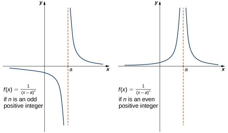 Figure 9. The function [latex]f(x)=1/(x-a)^n[/latex] has infinite limits at [latex]a[/latex].
Infinite Limits from Positive Integers
If [latex]n[/latex] is a positive even integer, then
If [latex]n[/latex] is a positive odd integer, then
and
We should also point out that in the graphs of [latex]f(x)=1/(x-a)^n[/latex], points on the graph having [latex]x[/latex]-coordinates very near to [latex]a[/latex] are very close to the vertical line [latex]x=a[/latex]. That is, as [latex]x[/latex] approaches [latex]a[/latex], the points on the graph of [latex]f(x)[/latex] are closer to the line [latex]x=a[/latex]. The line [latex]x=a[/latex] is called a vertical asymptote of the graph. We formally define a vertical asymptote as follows:
Definition
Let [latex]f(x)[/latex] be a function. If any of the following conditions hold, then the line [latex]x=a[/latex] is a vertical asymptote of [latex]f(x)[/latex]:
Finding a Vertical Asymptote
Evaluate each of the following limits using (Figure). Identify any vertical asymptotes of the function [latex]f(x)=1/(x+3)^4[/latex].
- [latex]\underset{x\to -3^-}{\lim}\frac{1}{(x+3)^4}[/latex]
- [latex]\underset{x\to -3^+}{\lim}\frac{1}{(x+3)^4}[/latex]
- [latex]\underset{x\to -3}{\lim}\frac{1}{(x+3)^4}[/latex]
Answer:
We can use (Figure) directly.
- [latex]\underset{x\to -3^-}{\lim}\frac{1}{(x+3)^4}=+\infty [/latex]
- [latex]\underset{x\to -3^+}{\lim}\frac{1}{(x+3)^4}=+\infty [/latex]
- [latex]\underset{x\to -3}{\lim}\frac{1}{(x+3)^4}=+\infty [/latex]
The function [latex]f(x)=1/(x+3)^4[/latex] has a vertical asymptote of [latex]x=-3[/latex].
Evaluate each of the following limits. Identify any vertical asymptotes of the function [latex]f(x)=\frac{1}{(x-2)^3}[/latex].
- [latex]\underset{x\to 2^-}{\lim}\frac{1}{(x-2)^3}[/latex]
- [latex]\underset{x\to 2^+}{\lim}\frac{1}{(x-2)^3}[/latex]
- [latex]\underset{x\to 2}{\lim}\frac{1}{(x-2)^3}[/latex]
Answer:
a. [latex]\underset{x\to 2^-}{\lim}\frac{1}{(x-2)^3}=−\infty[/latex];
b. [latex]\underset{x\to 2^+}{\lim}\frac{1}{(x-2)^3}=+\infty[/latex]; c. [latex]\underset{x\to 2}{\lim}\frac{1}{(x-2)^3}[/latex] DNE. The line [latex]x=2[/latex] is the vertical asymptote of [latex]f(x)=1/(x-2)^3[/latex].Hint
Use (Figure).
In the next example we put our knowledge of various types of limits to use to analyze the behavior of a function at several different points.
Behavior of a Function at Different Points
Use the graph of [latex]f(x)[/latex] in (Figure) to determine each of the following values:
- [latex]\underset{x\to 3^-}{\lim}f(x); \, \underset{x\to 3^+}{\lim}f(x); \, \underset{x\to 3}{\lim}f(x); \, f(3)[/latex]
- [latex]\underset{x\to \infty}{\lim}f(x)[/latex]
- [latex]\underset{x\to -\infty}{\lim}f(x)[/latex]
![The graph of a function f(x) described by the above limits and values. There is a smooth curve for values below x=-2; at (-2, 3), there is an open circle. There is a smooth curve between (-2, 1] with a closed circle at (1,6). There is an open circle at (1,3), and a smooth curve stretching from there down asymptotically to negative infinity along x=3. The function also curves asymptotically along x=3 on the other side, also stretching to negative infinity. The function then changes concavity in the first quadrant around y=4.5 and continues up.](https://s3-us-west-2.amazonaws.com/courses-images/wp-content/uploads/sites/2332/2018/01/11202918/CNX_Calc_Figure_02_02_015.jpg) Figure 10. The graph shows [latex]f(x)[/latex].
Figure 10. The graph shows [latex]f(x)[/latex].Answer:
Using (Figure) and the graph for reference, we arrive at the following values:
- [latex]\underset{x\to 3^-}{\lim}f(x)=−\infty; \, \underset{x\to 3^+}{\lim}f(x)=−\infty; \, \underset{x\to 3}{\lim}f(x)=-\infty; \, f(3)[/latex] is undefined
- [latex]\underset{x\to \infty}{\lim}f(x)=\infty[/latex]
- [latex]\underset{x\to -\infty}{\lim}f(x)=-\infty[/latex]
Evaluate [latex]\underset{x\to 1}{\lim}f(x)[/latex] for [latex]f(x)[/latex] shown here:
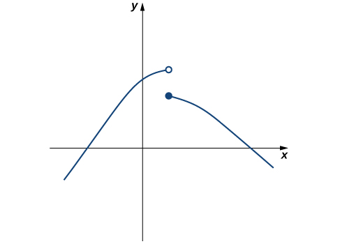
Answer:
Does not exist.
Hint
Compare the limit from the right with the limit from the left.
Limits at Infinity and Horizontal Asymptotes
Recall that [latex]\underset{x \to a}{\lim}f(x)=L[/latex] means [latex]f(x)[/latex] becomes arbitrarily close to [latex]L[/latex] as long as [latex]x[/latex] is sufficiently close to [latex]a[/latex]. We can extend this idea to limits at infinity. For example, consider the function [latex]f(x)=2+\frac{1}{x}[/latex]. As can be seen graphically in (Figure) and numerically in (Figure), as the values of [latex]x[/latex] get larger, the values of [latex]f(x)[/latex] approach 2. We say the limit as [latex]x[/latex] approaches [latex]\infty [/latex] of [latex]f(x)[/latex] is 2 and write [latex]\underset{x\to \infty }{\lim}f(x)=2[/latex]. Similarly, for [latex]x<0[/latex], as the values [latex]|x|[/latex] get larger, the values of [latex]f(x)[/latex] approaches 2. We say the limit as [latex]x[/latex] approaches [latex]−\infty [/latex] of [latex]f(x)[/latex] is 2 and write [latex]\underset{x\to a}{\lim}f(x)=2[/latex].
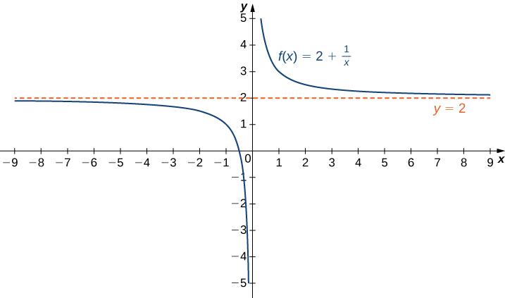 Figure 1. The function approaches the asymptote [latex]y=2[/latex] as [latex]x[/latex] approaches [latex]\pm \infty[/latex].
| [latex]x[/latex] | 10 | 100 | 1,000 | 10,000 |
| [latex]2+\frac{1}{x}[/latex] | 2.1 | 2.01 | 2.001 | 2.0001 |
| [latex]x[/latex] | -10 | -100 | -1000 | -10,000 |
| [latex]2+\frac{1}{x}[/latex] | 1.9 | 1.99 | 1.999 | 1.9999 |
More generally, for any function [latex]f[/latex], we say the limit as [latex]x \to \infty [/latex] of [latex]f(x)[/latex] is [latex]L[/latex] if [latex]f(x)[/latex] becomes arbitrarily close to [latex]L[/latex] as long as [latex]x[/latex] is sufficiently large. In that case, we write [latex]\underset{x\to a}{\lim}f(x)=L[/latex]. Similarly, we say the limit as [latex]x\to −\infty [/latex] of [latex]f(x)[/latex] is [latex]L[/latex] if [latex]f(x)[/latex] becomes arbitrarily close to [latex]L[/latex] as long as [latex]x<0[/latex] and [latex]|x|[/latex] is sufficiently large. In that case, we write [latex]\underset{x\to −\infty }{\lim}f(x)=L[/latex]. We now look at the definition of a function having a limit at infinity.
Definition
(Informal) If the values of [latex]f(x)[/latex] become arbitrarily close to [latex]L[/latex] as [latex]x[/latex] becomes sufficiently large, we say the function [latex]f[/latex] has a limit at infinity and write
If the values of [latex]f(x)[/latex] becomes arbitrarily close to [latex]L[/latex] for [latex]x<0[/latex] as [latex]|x|[/latex] becomes sufficiently large, we say that the function [latex]f[/latex] has a limit at negative infinity and write
If the values [latex]f(x)[/latex] are getting arbitrarily close to some finite value [latex]L[/latex] as [latex]x\to \infty [/latex] or [latex]x\to −\infty[/latex], the graph of [latex]f[/latex] approaches the line [latex]y=L[/latex]. In that case, the line [latex]y=L[/latex] is a horizontal asymptote of [latex]f[/latex] ((Figure)). For example, for the function [latex]f(x)=\frac{1}{x}[/latex], since [latex]\underset{x\to \infty }{\lim}f(x)=0[/latex], the line [latex]y=0[/latex] is a horizontal asymptote of [latex]f(x)=\frac{1}{x}[/latex].
Definition
If [latex]\underset{x\to \infty }{\lim}f(x)=L[/latex] or [latex]\underset{x \to −\infty}{\lim}f(x)=L[/latex], we say the line [latex]y=L[/latex] is a horizontal asymptote of [latex]f[/latex].
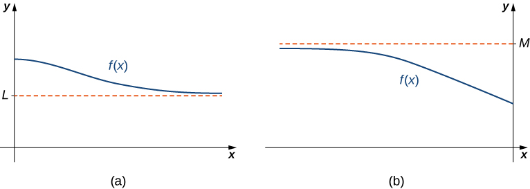 Figure 2. (a) As [latex]x\to \infty[/latex], the values of [latex]f[/latex] are getting arbitrarily close to [latex]L[/latex]. The line [latex]y=L[/latex] is a horizontal asymptote of [latex]f[/latex]. (b) As [latex]x\to −\infty[/latex], the values of [latex]f[/latex] are getting arbitrarily close to [latex]M[/latex]. The line [latex]y=M[/latex] is a horizontal asymptote of [latex]f[/latex].
A function cannot cross a vertical asymptote because the graph must approach infinity (or negative infinity) from at least one direction as [latex]x[/latex] approaches the vertical asymptote. However, a function may cross a horizontal asymptote. In fact, a function may cross a horizontal asymptote an unlimited number of times. For example, the function [latex]f(x)=\frac{ \cos x}{x}+1[/latex] shown in (Figure) intersects the horizontal asymptote [latex]y=1[/latex] an infinite number of times as it oscillates around the asymptote with ever-decreasing amplitude.
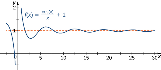 Figure 3. The graph of [latex]f(x)=\cos x/x+1[/latex] crosses its horizontal asymptote [latex]y=1[/latex] an infinite number of times.
The algebraic limit laws and squeeze theorem we introduced in Introduction to Limits also apply to limits at infinity. We illustrate how to use these laws to compute several limits at infinity.
Computing Limits at Infinity
For each of the following functions [latex]f[/latex], evaluate [latex]\underset{x\to \infty }{\lim}f(x)[/latex] and [latex]\underset{x\to −\infty }{\lim}f(x)[/latex]. Determine the horizontal asymptote(s) for [latex]f[/latex].
- [latex]f(x)=5-\frac{2}{x^2}[/latex]
- [latex]f(x)=\frac{\sin x}{x}[/latex]
- [latex]f(x)= \tan^{-1} (x)[/latex]
Answer:
- Using the algebraic limit laws, we have [latex]\underset{x\to \infty }{\lim}(5-\frac{2}{x^2})=\underset{x\to \infty }{\lim}5-2(\underset{x\to \infty }{\lim}\frac{1}{x})(\underset{x\to \infty }{\lim}\frac{1}{x})=5-2 \cdot 0=5[/latex]. Similarly, [latex]\underset{x\to \infty }{\lim}f(x)=5[/latex]. Therefore, [latex]f(x)=5-\frac{2}{x^2}[/latex] has a horizontal asymptote of [latex]y=5[/latex] and [latex]f[/latex] approaches this horizontal asymptote as [latex]x\to \pm \infty [/latex] as shown in the following graph.
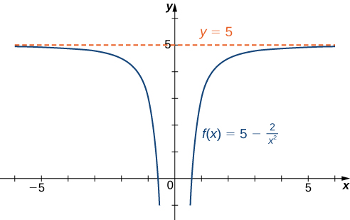 Figure 4. This function approaches a horizontal asymptote as [latex]x\to \pm \infty[/latex].
 - Since [latex]-1\le \sin x\le 1[/latex] for all [latex]x[/latex], we have
[latex]\frac{-1}{x}\le \frac{\sin x}{x}\le \frac{1}{x}[/latex]for all [latex]x \ne 0[/latex]. Also, since[latex]\underset{x\to \infty }{\lim}\frac{-1}{x}=0=\underset{x\to \infty }{\lim}\frac{1}{x}[/latex],we can apply the squeeze theorem to conclude that[latex]\underset{x\to \infty }{\lim}\frac{\sin x}{x}=0[/latex].Similarly,[latex]\underset{x\to −\infty}{\lim}\frac{\sin x}{x}=0[/latex].Thus, [latex]f(x)=\frac{\sin x}{x}[/latex] has a horizontal asymptote of [latex]y=0[/latex] and [latex]f(x)[/latex] approaches this horizontal asymptote as [latex]x\to \pm \infty [/latex] as shown in the following graph.
 Figure 5. This function crosses its horizontal asymptote multiple times.
 - To evaluate [latex]\underset{x\to \infty }{\lim} \tan^{-1} (x)[/latex] and [latex]\underset{x\to −\infty}{\lim} \tan^{-1} (x)[/latex], we first consider the graph of [latex]y= \tan (x)[/latex] over the interval [latex](−\pi /2,\pi /2)[/latex] as shown in the following graph.
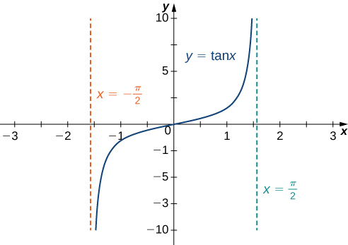 The graph of [latex] \tan x[/latex] has vertical asymptotes at [latex]x=\pm \frac{\pi }{2}[/latex]
Since
it follows that
Similarly, since
it follows that
As a result, [latex]y=\frac{\pi }{2}[/latex] and [latex]y=-\frac{\pi }{2}[/latex] are horizontal asymptotes of [latex]f(x)= \tan^{-1} (x)[/latex] as shown in the following graph.
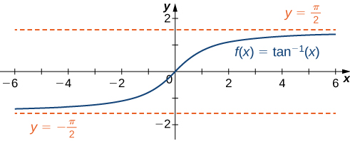 Figure 7. This function has two horizontal asymptotes.
Evaluate [latex]\underset{x\to −\infty}{\lim}(3+\frac{4}{x})[/latex] and [latex]\underset{x\to \infty }{\lim}(3+\frac{4}{x})[/latex]. Determine the horizontal asymptotes of [latex]f(x)=3+\frac{4}{x}[/latex], if any.
Answer:
Both limits are 3. The line [latex]y=3[/latex] is a horizontal asymptote.
Hint
[latex]\underset{x\to \pm \infty }{\lim}1/x=0[/latex]
Special Limits with Sine and Cosine
Definition
[latex]\underset{x\to \infty }{\lim}\sin x=DNE[/latex] [latex]\underset{x\to \infty }{\lim}\cos x=DNE[/latex] [latex]\underset{x\to \infty }{\lim}\frac{\sin x}{x}=\infty[/latex] [latex]\underset{x\to \infty }{\lim}\frac{\cos x}{x}=\infty[/latex]
Special limits with sine and cosine
For each of the following functions [latex]f[/latex], evaluate [latex]\underset{x\to \infty }{\lim}f(x)[/latex]
- [latex]f(x)=\frac{2-\sin x}{x}[/latex]
- [latex]f(x)=\sin\left(\frac{1}{x}\right)[/latex]
- [latex]f(x)= \frac{6}{5x-\cos x}[/latex]
Answer:
- Using the algebraic limit laws, we have [latex]\underset{x\to \infty }{\lim}\frac{2-\sin x}{x}=\underset{x\to \infty }{\lim}\frac{2x}{x}-\frac{\cos x}{x}=\underset{x\to \infty }{\lim}2-\frac{\cos x}{x}=\underset{x\to \infty }{\lim}2-\underset{x\to \infty }{\lim}\frac{\cos x}{x}=2-0=2[/latex].
- Since [latex]\underset{x\to \infty }{\lim}\frac{1}{x}=0[/latex], then [latex]\underset{x\to \infty }{\lim}\sin \left(\frac{1}{x} \right)=\sin(0)=0[/latex].
- Using the algebraic limit laws, we have [latex]\underset{x\to \infty }{\lim}\frac{6}{5x-\cos x}=\underset{x\to \infty }{\lim}\frac{\frac{6}{x}}{\frac{5x}{x}-\frac{\cos x}{x}}=\frac{\underset{x\to \infty }{\lim}\frac{6}{x}}{\underset{x\to \infty }{\lim}5-\underset{x\to \infty }{\lim}\frac{\cos x}{x}}=\frac{0}{5-0}=0[/latex].
Infinite Limits at Infinity
Sometimes the values of a function [latex]f[/latex] become arbitrarily large as [latex]x\to \infty [/latex] (or as [latex]x\to −\infty )[/latex]. In this case, we write [latex]\underset{x\to \infty }{\lim}f(x)=\infty [/latex] (or [latex]\underset{x\to −\infty }{\lim}f(x)=\infty )[/latex]. On the other hand, if the values of [latex]f[/latex] are negative but become arbitrarily large in magnitude as [latex]x\to \infty [/latex] (or as [latex]x\to −\infty )[/latex], we write [latex]\underset{x\to \infty }{\lim}f(x)=−\infty [/latex] (or [latex]\underset{x\to −\infty }{\lim}f(x)=−\infty )[/latex].
For example, consider the function [latex]f(x)=x^3[/latex]. As seen in (Figure) and (Figure), as [latex]x\to \infty [/latex] the values [latex]f(x)[/latex] become arbitrarily large. Therefore, [latex]\underset{x\to \infty }{\lim}x^3=\infty[/latex]. On the other hand, as [latex]x\to −\infty[/latex], the values of [latex]f(x)=x^3[/latex] are negative but become arbitrarily large in magnitude. Consequently, [latex]\underset{x\to −\infty }{\lim}x^3=−\infty[/latex].
| [latex]x[/latex] | 10 | 20 | 50 | 100 | 1000 |
| [latex]x^3[/latex] | 1000 | 8000 | 125,000 | 1,000,000 | 1,000,000,000 |
| [latex]x[/latex] | -10 | -20 | -50 | -100 | -1000 |
| [latex]x^3[/latex] | -1000 | -8000 | -125,000 | -1,000,000 | -1,000,000,000 |
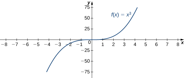 Figure 8. For this function, the functional values approach infinity as [latex]x\to \pm \infty[/latex].
Definition
(Informal) We say a function [latex]f[/latex] has an infinite limit at infinity and write
if [latex]f(x)[/latex] becomes arbitrarily large for [latex]x[/latex] sufficiently large. We say a function has a negative infinite limit at infinity and write
if [latex]f(x)<0[/latex] and [latex]|f(x)|[/latex] becomes arbitrarily large for [latex]x[/latex] sufficiently large. Similarly, we can define infinite limits as [latex]x\to −\infty[/latex].
Formal Definitions
Earlier, we used the terms arbitrarily close, arbitrarily large, and sufficiently large to define limits at infinity informally. Although these terms provide accurate descriptions of limits at infinity, they are not precise mathematically. Here are more formal definitions of limits at infinity. We then look at how to use these definitions to prove results involving limits at infinity.
Definition
(Formal) We say a function [latex]f[/latex] has a limit at infinity, if there exists a real number [latex]L[/latex] such that for all [latex]\epsilon >0[/latex], there exists [latex]N>0[/latex] such that
for all [latex]x>N[/latex]. In that case, we write
(see (Figure)).
We say a function [latex]f[/latex] has a limit at negative infinity if there exists a real number [latex]L[/latex] such that for all [latex]\epsilon >0[/latex], there exists [latex]N<0[/latex] such that
for all [latex]x<N[/latex]. In that case, we write
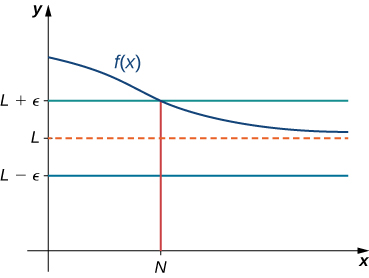 Figure 9. For a function with a limit at infinity, for all [latex]x>N[/latex], [latex]|f(x)-L|<\epsilon [/latex].
Earlier in this section, we used graphical evidence in (Figure) and numerical evidence in (Figure) to conclude that [latex]\underset{x\to \infty }{\lim}(\frac{2+1}{x})=2[/latex]. Here we use the formal definition of limit at infinity to prove this result rigorously.
A Finite Limit at Infinity Example
Use the formal definition of limit at infinity to prove that [latex]\underset{x\to \infty }{\lim}(2+\frac{1}{x})=2[/latex].
Answer:
Let [latex]\epsilon >0[/latex]. Let [latex]N=\frac{1}{\epsilon }[/latex]. Therefore, for all [latex]x>N[/latex], we have
Use the formal definition of limit at infinity to prove that [latex]\underset{x\to \infty }{\lim}(3 - \frac{1}{x^2})=3[/latex].
Answer:
Let [latex]\epsilon >0[/latex]. Let [latex]N=\frac{1}{\sqrt{\epsilon }}[/latex]. Therefore, for all [latex]x>N[/latex], we have
[latex]|3-\frac{1}{x^2}-3|=\frac{1}{x^2}<\frac{1}{N^2}=\epsilon [/latex]
Therefore, [latex]\underset{x\to \infty }{\lim}(3-1/x^2)=3[/latex].
Hint
Let [latex]N=\frac{1}{\sqrt{\epsilon }}[/latex].
We now turn our attention to a more precise definition for an infinite limit at infinity.
Definition
(Formal) We say a function [latex]f[/latex] has an infinite limit at infinity and write
if for all [latex]M>0[/latex], there exists an [latex]N>0[/latex] such that
for all [latex]x>N[/latex] (see (Figure)).
We say a function has a negative infinite limit at infinity and write
if for all [latex]M<0[/latex], there exists an [latex]N>0[/latex] such that
for all [latex]x>N[/latex].
Similarly we can define limits as [latex]x\to −\infty[/latex].
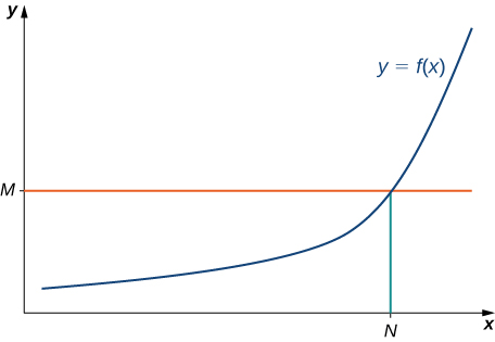 Figure 10. For a function with an infinite limit at infinity, for all [latex]x>N[/latex], [latex]f(x)>M[/latex].
Earlier, we used graphical evidence ((Figure)) and numerical evidence ((Figure)) to conclude that [latex]\underset{x\to \infty }{\lim}x^3=\infty[/latex]. Here we use the formal definition of infinite limit at infinity to prove that result.
An Infinite Limit at Infinity
Use the formal definition of infinite limit at infinity to prove that [latex]\underset{x\to \infty }{\lim}x^3=\infty[/latex].
Answer:
Let [latex]M>0[/latex]. Let [latex]N=\sqrt[3]{M}[/latex]. Then, for all [latex]x>N[/latex], we have
Therefore, [latex]\underset{x\to \infty }{\lim}x^3=\infty[/latex].
Use the formal definition of infinite limit at infinity to prove that [latex]\underset{x\to \infty }{\lim}3x^2=\infty[/latex].
Answer:
Let [latex]M>0[/latex]. Let [latex]N=\sqrt{\frac{M}{3}}[/latex]. Then, for all [latex]x>N[/latex], we have
[latex]3x^2>3N^2=3(\sqrt{\frac{M}{3}})^2=\frac{3M}{3}=M[/latex]
Hint
Let [latex]N=\sqrt{\frac{M}{3}}[/latex].
Key Equations
- Infinite Limits from the Left [latex-display]\underset{x\to a^-}{\lim}f(x)=+\infty[/latex-display] [latex]\underset{x\to a^-}{\lim}f(x)=−\infty [/latex]
- Infinite Limits from the Right [latex-display]\underset{x\to a^+}{\lim}f(x)=+\infty[/latex-display] [latex]\underset{x\to a^+}{\lim}f(x)=−\infty [/latex]
- Two-Sided Infinite Limits [latex-display]\underset{x\to a}{\lim}f(x)=+\infty: \underset{x\to a^-}{\lim}f(x)=+\infty[/latex] and [latex]\underset{x\to a^+}{\lim}f(x)=+\infty[/latex-display] [latex]\underset{x\to a}{\lim}f(x)=−\infty: \underset{x\to a^-}{\lim}f(x)=−\infty [/latex] and [latex]\underset{x\to a^+}{\lim}f(x)=−\infty [/latex]
In the following exercises, use direct substitution to obtain an undefined expression. Then, use the method of (Figure) to simplify the function to help determine the limit.
1. [latex]\underset{x\to -2^-}{\lim}\frac{2x^2+7x-4}{x^2+x-2}[/latex]
Answer:
[latex]-\infty[/latex]
2. [latex]\underset{x\to -2^+}{\lim}\frac{2x^2+7x-4}{x^2+x-2}[/latex]
3. [latex]\underset{x\to 1^-}{\lim}\frac{2x^2+7x-4}{x^2+x-2}[/latex]
Answer:
[latex]-\infty[/latex]
4. [latex]\underset{x\to 1^+}{\lim}\frac{2x^2+7x-4}{x^2+x-2}[/latex]
For the following exercises, evaluate the limit.
5. [latex]\underset{x\to \infty }{\lim}\frac{1}{3x+6}[/latex]
Answer:
0
6. [latex]\underset{x\to \infty }{\lim}\frac{2x-5}{4x}[/latex]
7. [latex]\underset{x\to \infty }{\lim}\frac{x^2-2x+5}{x+2}[/latex]
Answer:
[latex]\infty [/latex]
8. [latex]\underset{x\to −\infty }{\lim}\frac{3x^3-2x}{x^2+2x+8}[/latex]
9. [latex]\underset{x\to −\infty }{\lim}\frac{x^4-4x^3+1}{2-2x^2-7x^4}[/latex]
Answer:
[latex]-\frac{1}{7}[/latex]
10. [latex]\underset{x\to \infty }{\lim}\frac{3x}{\sqrt{x^2+1}}[/latex]
11. [latex]\underset{x\to −\infty }{\lim}\frac{\sqrt{4x^2-1}}{x+2}[/latex]
Answer:
-2
12. [latex]\underset{x\to \infty }{\lim}\frac{4x}{\sqrt{x^2-1}}[/latex]
13. [latex]\underset{x\to −\infty }{\lim}\frac{4x}{\sqrt{x^2-1}}[/latex]
Answer:
-4
14. [latex]\underset{x\to \infty }{\lim}\frac{2\sqrt{x}}{x-\sqrt{x}+1}[/latex]
For the following exercises, find the horizontal and vertical asymptotes.
15. [latex]f(x)=x-\frac{9}{x}[/latex]
Answer:
Horizontal: none, vertical: [latex]x=0[/latex]
16. [latex]f(x)=\frac{1}{1-x^2}[/latex]
17. [latex]f(x)=\frac{x^3}{4-x^2}[/latex]
Answer:
Horizontal: none, vertical: [latex]x=\pm 2[/latex]
18. [latex]f(x)=\frac{x^2+3}{x^2+1}[/latex]
19. [latex]f(x)= \sin (x) \sin (2x)[/latex]
Answer:
Horizontal: none, vertical: none
20. [latex]f(x)= \cos x+ \cos (3x)+ \cos (5x)[/latex]
21. [latex]f(x)=\frac{x \sin (x)}{x^2-1}[/latex]
Answer:
Horizontal: [latex]y=0[/latex], vertical: [latex]x=\pm 1[/latex]
[latex]f(x)=\frac{x}{ \sin (x)}[/latex]
22. [latex]f(x)=\frac{1}{x^3+x^2}[/latex]
Answer:
Horizontal: [latex]y=0[/latex], vertical: [latex]x=0[/latex] and [latex]x=-1[/latex]
23. [latex]f(x)=\frac{1}{x-1}-2x[/latex]
24. [latex]f(x)=\frac{x^3+1}{x^3-1}[/latex]
Answer:
Horizontal: [latex]y=1[/latex], vertical: [latex]x=1[/latex]
25. [latex]f(x)=\frac{ \sin x+ \cos x}{ \sin x- \cos x}[/latex]
26. [latex]f(x)=x- \sin x[/latex]
Answer:
Horizontal: none, vertical: none
27. [latex]f(x)=\frac{1}{x}-\sqrt{x}[/latex]
In the following exercises, sketch the graph of a function with the given properties.
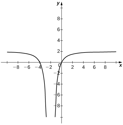
28. [latex]\underset{x\to -\infty }{\lim}f(x)=0, \, \underset{x\to -1^-}{\lim}f(x)=−\infty[/latex], [latex]\underset{x\to -1^+}{\lim}f(x)=\infty, \, \underset{x\to 0}{\lim}f(x)=f(0), \, f(0)=1, \, \underset{x\to \infty }{\lim}f(x)=−\infty [/latex]
Answer:
Answers may vary.
29. [latex]\underset{x\to -\infty}{\lim}f(x)=2, \, \underset{x\to 3^-}{\lim}f(x)=−\infty[/latex], [latex]\underset{x\to 3^+}{\lim}f(x)=\infty, \, \underset{x\to \infty }{\lim}f(x)=2, \, f(0)=\frac{-1}{3}[/latex]
30. [latex]\underset{x\to -\infty }{\lim}f(x)=2, \, \underset{x\to -2}{\lim}f(x)=−\infty[/latex],[latex]\underset{x\to \infty }{\lim}f(x)=2, \, f(0)=0[/latex]
Answer:
Answers may vary.
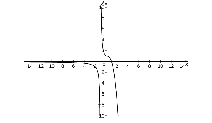
31. [latex]\underset{x\to -\infty }{\lim}f(x)=0, \, \underset{x\to -1^-}{\lim}f(x)=\infty, \, \underset{x\to -1^+}{\lim}f(x)=−\infty, \, f(0)=-1, \, \underset{x\to 1^-}{\lim}f(x)=−\infty, \, \underset{x\to 1^+}{\lim}f(x)=\infty, \, \underset{x\to \infty }{\lim}f(x)=0[/latex]
32. [T] In physics, the magnitude of an electric field generated by a point charge at a distance [latex]r[/latex] in vacuum is governed by Coulomb’s law: [latex]E(r)=\large \frac{q}{4\pi \epsilon_0 r^2}[/latex], where [latex]E[/latex] represents the magnitude of the electric field, [latex]q[/latex] is the charge of the particle, [latex]r[/latex] is the distance between the particle and where the strength of the field is measured, and [latex]\large \frac{1}{4\pi \epsilon_0}[/latex] is Coulomb’s constant: [latex]8.988 \times 10^9 \, \text{N} \cdot \text{m}^2/\text{C}^2[/latex].
- Use a graphing calculator to graph [latex]E(r)[/latex] given that the charge of the particle is [latex]q=10^{-10}[/latex].
- Evaluate [latex]\underset{r\to 0^+}{\lim}E(r)[/latex]. What is the physical meaning of this quantity? Is it physically relevant? Why are you evaluating from the right?
Answer:
a.
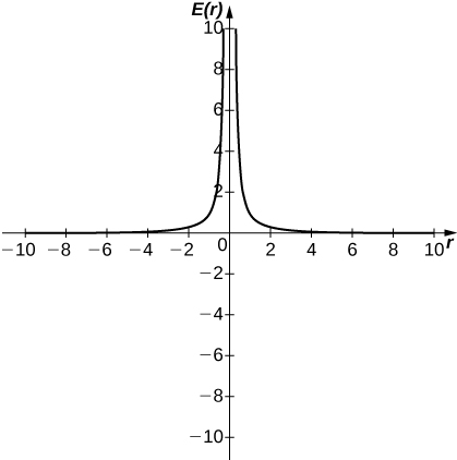 b. [latex]\underset{r\to 0^+}{\lim}E(r)=\infty[/latex]. The magnitude of the electric field as you approach the particle [latex]q[/latex] becomes infinite. It does not make physical sense to evaluate negative distance.
33. [T] The density of an object is given by its mass divided by its volume: [latex]\rho =m/V[/latex].
- Use a calculator to plot the volume as a function of density [latex](V=m/\rho)[/latex], assuming you are examining something of mass 8 kg ([latex]m=8[/latex]).
- Evaluate [latex]\underset{\rho \to 0^+}{\lim}V(\rho)[/latex] and explain the physical meaning.
Licenses & Attributions
CC licensed content, Shared previously
- Calculus I. Provided by: OpenStax Located at: https://openstax.org/books/calculus-volume-1/pages/1-introduction. License: CC BY-NC-SA: Attribution-NonCommercial-ShareAlike. License terms: Download for free at http://cnx.org/contents/[email protected].

Hint
Follow the procedures from (Figure).