Graph Polynomial Functions
Learning Objectives
- Draw the graph of a polynomial function using end behavior, turning points, intercepts, and the intermediate value theorem
How To: Given a polynomial function, sketch the graph.
- Find the intercepts.
- Check for symmetry. If the function is an even function, its graph is symmetrical about the y-axis, that is, f(–x) = f(x). If a function is an odd function, its graph is symmetrical about the origin, that is, f(–x) = –f(x).
- Use the multiplicities of the zeros to determine the behavior of the polynomial at the x-intercepts.
- Determine the end behavior by examining the leading term.
- Use the end behavior and the behavior at the intercepts to sketch a graph.
- Ensure that the number of turning points does not exceed one less than the degree of the polynomial.
- Optionally, use technology to check the graph.
Example: Sketching the Graph of a Polynomial Function
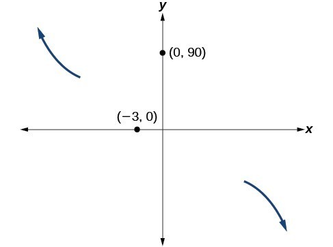
Sketch a graph of [latex]f\left(x\right)=-2{\left(x+3\right)}^{2}\left(x - 5\right)[/latex].Answer: This graph has two x-intercepts. At x = –3, the factor is squared, indicating a multiplicity of 2. The graph will bounce at this x-intercept. At x = 5, the function has a multiplicity of one, indicating the graph will cross through the axis at this intercept. The y-intercept is found by evaluating f(0).
[latex]\begin{array}{l}\hfill \\ f\left(0\right)=-2{\left(0+3\right)}^{2}\left(0 - 5\right)\hfill \\ \text{ }=-2\cdot 9\cdot \left(-5\right)\hfill \\ \text{ }=90\hfill \end{array}[/latex]
The y-intercept is (0, 90).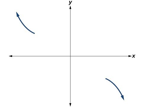 Additionally, we can see the leading term, if this polynomial were multiplied out, would be [latex]-2{x}^{3}[/latex], so the end behavior is that of a vertically reflected cubic, with the outputs decreasing as the inputs approach infinity, and the outputs increasing as the inputs approach negative infinity.
To sketch this, we consider that:
Additionally, we can see the leading term, if this polynomial were multiplied out, would be [latex]-2{x}^{3}[/latex], so the end behavior is that of a vertically reflected cubic, with the outputs decreasing as the inputs approach infinity, and the outputs increasing as the inputs approach negative infinity.
To sketch this, we consider that:
- As [latex]x\to -\infty [/latex] the function [latex]f\left(x\right)\to \infty [/latex], so we know the graph starts in the second quadrant and is decreasing toward the x-axis.
- Since [latex]f\left(-x\right)=-2{\left(-x+3\right)}^{2}\left(-x - 5\right)[/latex] is not equal to f(x), the graph does not display symmetry.
- At [latex]\left(-3,0\right)[/latex], the graph bounces off of the x-axis, so the function must start increasing.At (0, 90), the graph crosses the y-axis at the y-intercept.
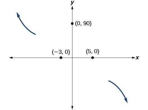 Somewhere after this point, the graph must turn back down or start decreasing toward the horizontal axis because the graph passes through the next intercept at (5, 0).
As [latex]x\to \infty [/latex] the function [latex]f\left(x\right)\to \mathrm{-\infty }[/latex], so we know the graph continues to decrease, and we can stop drawing the graph in the fourth quadrant.
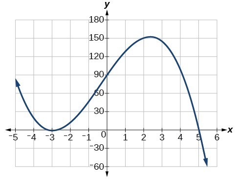
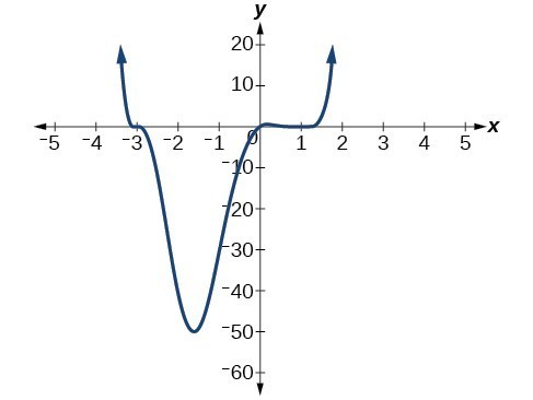
Using technology, we can create the graph for the polynomial function, shown in Figure 16, and verify that the resulting graph looks like our sketch in Figure 15.
The complete graph of the polynomial function [latex]f\left(x\right)=-2{\left(x+3\right)}^{2}\left(x - 5\right)[/latex]
Somewhere after this point, the graph must turn back down or start decreasing toward the horizontal axis because the graph passes through the next intercept at (5, 0).
As [latex]x\to \infty [/latex] the function [latex]f\left(x\right)\to \mathrm{-\infty }[/latex], so we know the graph continues to decrease, and we can stop drawing the graph in the fourth quadrant.
Using technology, we can create the graph for the polynomial function, shown in Figure 16, and verify that the resulting graph looks like our sketch in Figure 15.
The complete graph of the polynomial function [latex]f\left(x\right)=-2{\left(x+3\right)}^{2}\left(x - 5\right)[/latex]
Try It
Sketch a graph of [latex]f\left(x\right)=\frac{1}{4}x{\left(x - 1\right)}^{4}{\left(x+3\right)}^{3}[/latex]. Check yourself with Desmos when you are done.Answer:
Try it
Use Desmos to write an odd degree function with one zero at (-3,0) whose multiplicity is 3 and another zero at (2,0) with multiplicity 2. The end behavior of the graph is: as [latex]x\rightarrow-\infty, f(x) \rightarrow\infty[/latex] and as [latex]x\rightarrow \infty, f(x)\rightarrow -\infty[/latex]The Intermediate Value Theorem
In some situations, we may know two points on a graph but not the zeros. If those two points are on opposite sides of the x-axis, we can confirm that there is a zero between them. Consider a polynomial function f whose graph is smooth and continuous. The Intermediate Value Theorem states that for two numbers a and b in the domain of f, if a < b and [latex]f\left(a\right)\ne f\left(b\right)[/latex], then the function f takes on every value between [latex]f\left(a\right)[/latex] and [latex]f\left(b\right)[/latex]. We can apply this theorem to a special case that is useful in graphing polynomial functions. If a point on the graph of a continuous function f at [latex]x=a[/latex] lies above the x-axis and another point at [latex]x=b[/latex] lies below the x-axis, there must exist a third point between [latex]x=a[/latex] and [latex]x=b[/latex] where the graph crosses the x-axis. Call this point [latex]\left(c,\text{ }f\left(c\right)\right)[/latex]. This means that we are assured there is a solution c where [latex]f\left(c\right)=0[/latex]. In other words, the Intermediate Value Theorem tells us that when a polynomial function changes from a negative value to a positive value, the function must cross the x-axis. The figure below shows that there is a zero between a and b.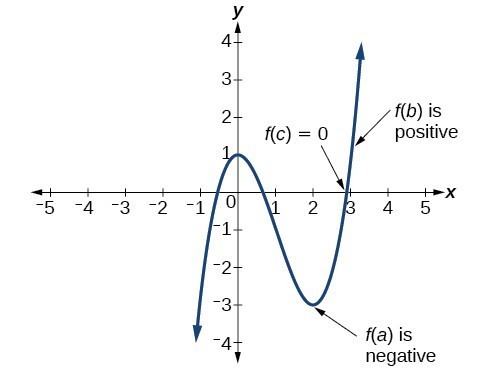 Using the Intermediate Value Theorem to show there exists a zero.
A General Note: Intermediate Value Theorem
Let f be a polynomial function. The Intermediate Value Theorem states that if [latex]f\left(a\right)[/latex] and [latex]f\left(b\right)[/latex] have opposite signs, then there exists at least one value c between a and b for which [latex]f\left(c\right)=0[/latex].Example: Using the Intermediate Value Theorem
Show that the function [latex]f\left(x\right)={x}^{3}-5{x}^{2}+3x+6[/latex] has at least two real zeros between [latex]x=1[/latex] and [latex]x=4[/latex].Answer: As a start, evaluate [latex]f\left(x\right)[/latex] at the integer values [latex]x=1,2,3,\text{ and }4[/latex].
| x | 1 | 2 | 3 | 4 |
| f (x) | 5 | 0 | –3 | 2 |
Analysis of the Solution
We can also see that there are two real zeros between [latex]x=1[/latex] and [latex]x=4[/latex].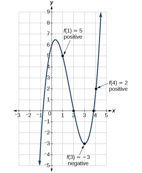
Try It
Show that the function [latex]f\left(x\right)=7{x}^{5}-9{x}^{4}-{x}^{2}[/latex] has at least one real zero between [latex]x=1[/latex] and [latex]x=2[/latex].Answer: Because f is a polynomial function and since [latex]f\left(1\right)[/latex] is negative and [latex]f\left(2\right)[/latex] is positive, there is at least one real zero between [latex]x=1[/latex] and [latex]x=2[/latex].
Licenses & Attributions
CC licensed content, Original
- Interactive: Write a Polynomial Function. Provided by: Lumen Learning (With Desmos) License: CC BY: Attribution.
- Revision and Adaptation. Provided by: Lumen Learning License: CC BY: Attribution.
CC licensed content, Shared previously
- College Algebra. Provided by: OpenStax Authored by: Abramson, Jay et al.. Located at: https://openstax.org/books/college-algebra/pages/1-introduction-to-prerequisites. License: CC BY: Attribution. License terms: Download for free at http://cnx.org/contents/[email protected].
