O.05: Section 3
Section 3: Composite models—Using different formulas for different parts of the graph
Compound models add two or more modeling functions together. The other main way in which models are combined is to “compose” a new model by using different modeling formulas depending on what the input values are. The graphs of such composite models will usually have a sharp break, in value or slope or both, at each point in the input range at which there is a switch from one function to another. Income taxes due are described by a composite model with a change in slope for each tax bracket. In this case each piece of the model is a straight line segment starting at the end of the previous one.
Each segment of a composite model can be built of any kind of modeling formula. The model output can have abrupt jumps in value, although it is more usual for changes at the transition values to be in the slope, since few processes have big output changes for small input changes. Sometimes the position of the transition between formulas is a parameter of the model, so that the fitting process lets the data tell you where the transition is. In the common situation where the transition is at the intersection of two fitted formulas, the transition can usually be deduced algebraically by setting the two formulas equal to each other (using the fitted parameters as coefficients) and solving for the x and y of the crossing point.
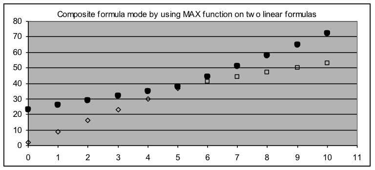
Two main approaches are used to “composing” a composite model. The simplest approach is to use each input value to evaluate two or more formulas, then pick the largest of the results to use as the output value. The effect is to make a model whose graph follows the top of the graphs of each of the component formulas. This can be implemented in a spreadsheet with the MAX function, whose value is equal to the largest of its arguments (e.g., the value of “=MAX(14,22,-30,5)” is 22).
The graph and table below show the output of a model formula that uses two linear formulas (y=3x+23 and y=7x+2) as arguments to the MAX function. The solid circles are the output of the composite model that results from the MAX function, while the empty triangles and squares show the portions of the two linear formulas that are not used because the other formula is larger at that x value.
Income taxes due are described by a composite model with a change in slope for each tax bracket. In this case each piece of the model is a straight line segment starting at the end of the previous one.
Each segment of a composite model can be built of any kind of modeling formula. The model output can have abrupt jumps in value, although it is more usual for changes at the transition values to be in the slope, since few processes have big output changes for small input changes. Sometimes the position of the transition between formulas is a parameter of the model, so that the fitting process lets the data tell you where the transition is. In the common situation where the transition is at the intersection of two fitted formulas, the transition can usually be deduced algebraically by setting the two formulas equal to each other (using the fitted parameters as coefficients) and solving for the x and y of the crossing point.
Two main approaches are used to “composing” a composite model. The simplest approach is to use each input value to evaluate two or more formulas, then pick the largest of the results to use as the output value. The effect is to make a model whose graph follows the top of the graphs of each of the component formulas. This can be implemented in a spreadsheet with the MAX function, whose value is equal to the largest of its arguments (e.g., the value of “=MAX(14,22,-30,5)” is 22).
The graph and table below show the output of a model formula that uses two linear formulas (y=3x+23 and y=7x+2) as arguments to the MAX function. The solid circles are the output of the composite model that results from the MAX function, while the empty triangles and squares show the portions of the two linear formulas that are not used because the other formula is larger at that x value.
|
 |
| Example 5: A cylindrical water tank drains through two outlets, one near the bottom of the tank and the other near the middle. Each outlet pumps at a steady (but different) rate until the water drops below the opening to its outlet. The dataset to the right shows the water depth measured in feet at one-minute intervals during drainage. Based on this data, find the answer to these questions: [a] What percentage of the total pumping capacity is provided by the outlet at the bottom of the tank? [b] What is the depth of the tank at its upper outlet? |
|
[latex]\begin{align}&\text{At the crossing point,}{{y}_{cross}}=53.27-8.23{{x}_{cross}}\text{ and }{{y}_{cross}}=33.46-2.37{{x}_{cross}}\\&\text{Therefore: }53.27-8.23{{x}_{cross}}=33.46-2.37{{x}_{cross}}\\&\text{}-8.23{{x}_{cross}}+2.37{{x}_{cross}}=33.46-53.27\\&\text{}-5.86{{x}_{cross}}=-19.81\\&\text{}{{x}_{cross}}=3.3805\text{ minutes}\\&\text{So}{{y}_{cross}}=53.27-8.23{{x}_{cross}}=53.27-8.23\cdot3.3805=53.27-27.82=25.45\text{ feet}\\\end{align}[/latex]
Best-fit Solver results| 53.27 | Intercept 1 |
| -8.23 | Slope 1 |
| 33.46 | Intercept 2 |
| -2.37 | Slope 2 |
Licenses & Attributions
CC licensed content, Shared previously
- Mathematics for Modeling. Authored by: Mary Parker and Hunter Ellinger. License: CC BY: Attribution.
