Inverse Functions: Exponential, Logarithmic, and Trigonometric Functions
Inverse Functions
An inverse function is a function that undoes another function.Learning Objectives
Discuss what it means to be an inverse functionKey Takeaways
Key Points
- If an input [latex]x[/latex] into the function [latex]f[/latex] produces an output [latex]y[/latex], then putting [latex]y[/latex] into the inverse function [latex]g[/latex] produces the output [latex]x[/latex], and vice versa (i.e., [latex]f(x)=y[/latex], and [latex]g(y)=x[/latex]).
- A function [latex]f[/latex] that has an inverse is called invertible; the inverse function is then uniquely determined by [latex]f[/latex] and is denoted by [latex]f^{-1}[/latex].
- If [latex]f[/latex] is invertible, the function [latex]g[/latex] is unique; in other words, there is exactly one function [latex]g[/latex] satisfying this property (no more, no fewer).
Key Terms
- inverse: a function that undoes another function
- function: a relation in which each element of the domain is associated with exactly one element of the co-domain
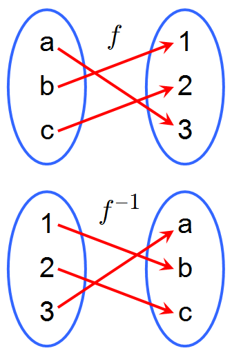
A Function and its Inverse: A function [latex]f[/latex] and its inverse, [latex]f^{-1}[/latex]. Because [latex]f[/latex] maps [latex]a[/latex] to [latex]3[/latex], the inverse [latex]f^{-1}[/latex] maps [latex]3[/latex] back to [latex]a[/latex].
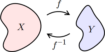
Inverse Functions: If [latex]f[/latex] maps [latex]X[/latex] to [latex]Y[/latex], then [latex]f^{-1}[/latex] maps [latex]Y[/latex] back to [latex]X[/latex].
Example
Let's take the function [latex]y=x^2+2[/latex]. To find the inverse of this function, undo each of the operations on the [latex]x[/latex] side of the equation one at a time. We start with the [latex]+2[/latex] operation. Notice that we start in the opposite order of the normal order of operations when we undo operations. The opposite of [latex]+2[/latex] is [latex]-2[/latex]. We are left with [latex]x^2[/latex]. To undo use the square root operation. Thus, the inverse of [latex]x^2+2[/latex] is [latex]\sqrt{x-2}[/latex]. We can check to see if this inverse "undoes" the original function by plugging that function in for [latex]x[/latex]: [latex-display]\sqrt{\left(x^2+2\right)-2}=\sqrt{x^2}=x[/latex-display]Derivatives of Exponential Functions
The derivative of the exponential function is equal to the value of the function.Learning Objectives
Solve for the derivatives of exponential functionsKey Takeaways
Key Points
- [latex]e^x[/latex] is its own derivative: [latex]\frac{d}{dx}e^{x} = e^{x}[/latex].
- If a variable 's growth or decay rate is proportional to its size, then the variable can be written as a constant times an exponential function of time.
- For any differentiable function [latex]f(x)[/latex], [latex]\frac{d}{dx}e^{f(x)} = f'(x)e^{f(x)}[/latex].
Key Terms
- exponential: any function that has an exponent as an independent variable
- tangent: a straight line touching a curve at a single point without crossing it there
- e: the base of the natural logarithm, [latex]2.718281828459045\dots[/latex]

Graph of an Exponential Function: Graph of the exponential function illustrating that its derivative is equal to the value of the function. From any point [latex]P[/latex] on the curve (blue), let a tangent line (red), and a vertical line (green) with height [latex]h[/latex] be drawn, forming a right triangle with a base [latex]b[/latex] on the [latex]x[/latex]-axis. Since the slope of the red tangent line (the derivative) at [latex]P[/latex] is equal to the ratio of the triangle's height to the triangle's base (rise over run), and the derivative is equal to the value of the function, [latex]h[/latex] must be equal to the ratio of [latex]h[/latex] to [latex]b[/latex]. Therefore, the base [latex]b[/latex] must always be [latex]1[/latex].
- The slope of the graph at any point is the height of the function at that point.
- The rate of increase of the function at [latex]x[/latex] is equal to the value of the function at [latex]x[/latex].
- The function solves the differential equation [latex]y' = y [/latex].
- [latex]e^x[/latex] is a fixed point of derivative as a functional.
Logarithmic Functions
The logarithm of a number is the exponent by which another fixed value must be raised to produce that number.Learning Objectives
Demonstrate that logarithmic functions are the inverses of exponential functionsKey Takeaways
Key Points
- The idea of logarithms is to reverse the operation of exponentiation, that is raising a number to a power.
- A naive way of defining the logarithm of a number [latex]x[/latex] with respect to base [latex]b[/latex] is the exponent by which [latex]b[/latex] must be raised to yield [latex]x[/latex].
- To define the logarithm, the base [latex]b[/latex] must be a positive real number not equal to [latex]1[/latex] and [latex]x[/latex] must be a positive number.
Key Terms
- binary: the bijective base-2 numeral system, which uses only the digits 0 and 1
- exponent: the power to which a number, symbol or expression is to be raised: for example, the [latex]3[/latex] in [latex]x^3[/latex].
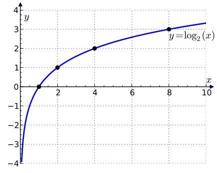
Plot of [latex]\log_2(x)[/latex]: The graph of the logarithm to base 2 crosses the x-axis (horizontal axis) at 1 and passes through the points with coordinates (2, 1), (4, 2), and (8, 3). For example, log2(8) = 3, because 23 = 8. The graph gets arbitrarily close to the y axis, but does not meet or intersect it.
Derivatives of Logarithmic Functions
The general form of the derivative of a logarithmic function is [latex]\frac{d}{dx}\log_{b}(x) = \frac{1}{xln(b)}[/latex].Learning Objectives
Solve for the derivative of a logarithmic functionKey Takeaways
Key Points
- The derivative of natural logarithmic function is [latex]\frac{d}{dx}\ln(x) = \frac{1}{x}[/latex].
- The general form of the derivative of a logarithmic function can be derived from the derivative of a natural logarithmic function.
- Properties of the logarithm can be used to to differentiate more difficult functions, such as products with many terms, quotients of composed functions, or functions with variable or function exponents.
Key Terms
- logarithm: the exponent by which another fixed value, the base, must be raised to produce that number
- e: the base of the natural logarithm, [latex]2.718281828459045\dots[/latex]
- [latex]\log \left(\dfrac{a}{b}\right) = \log (a) - \log (b)[/latex]
- [latex]\log(a^{n}) = n \log(a)[/latex]
- [latex]\log(a) + \log (b) = \log(ab)[/latex]
The Natural Logarithmic Function: Differentiation and Integration
Differentiation and integration of natural logarithms is based on the property [latex]\frac{d}{dx}\ln(x) = \frac{1}{x}[/latex].Learning Objectives
Practice integrating and differentiating the natural logarithmic functionKey Takeaways
Key Points
- The natural logarithm allows simple integration of functions of the form [latex]g(x) = \frac{ f '(x)}{f(x)}[/latex].
- The natural logarithm can be integrated using integration by parts: [latex]\int\ln(x)dx=x \ln(x)−x+C[/latex].
- The derivative of the natural logarithm leads to the Taylor series for [latex]\ln(1 + x)[/latex] around [latex]0[/latex]: [latex]\ln(1+x) = x - \frac{x^{2}}{2} + \frac{x^{3}}{3} - \cdots[/latex] for [latex]\left | x \right | \leq 1[/latex] (unless [latex]x = -1[/latex]).
Key Terms
- transcendental: of or relating to a number that is not the root of any polynomial that has positive degree and rational coefficients
- irrational: of a real number, that cannot be written as the ratio of two integers
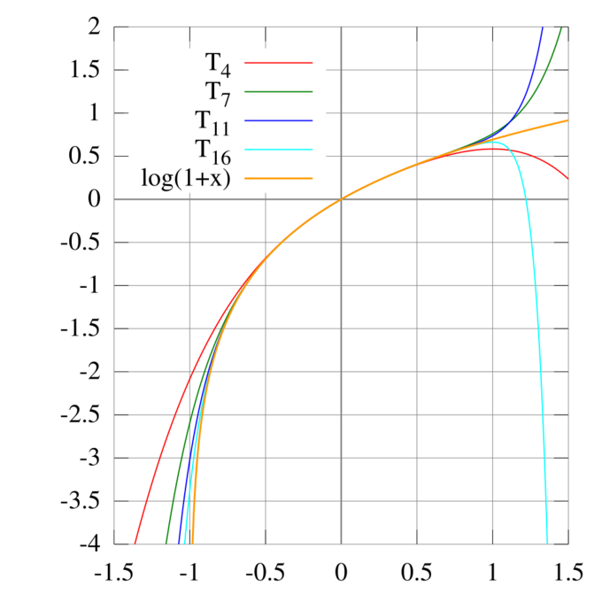
Taylor Series Approximations for [latex]\ln(1+x)[/latex]: The Taylor polynomials for [latex]\ln(1 + x)[/latex] only provide accurate approximations in the range [latex]-1 < x \leq 1[/latex]. Note that, for [latex]x>1[/latex], the Taylor polynomials of higher degree are worse approximations.
The Natural Exponential Function: Differentiation and Integration
The derivative of the exponential function [latex]\frac{d}{dx}a^x = \ln(a)a^{x}[/latex].Learning Objectives
Practice integrating and differentiating the natural exponential functionKey Takeaways
Key Points
- The formula for differentiation of exponential function [latex]a^{x}[/latex] can be derived from a specific case of natural exponential function [latex]e^{x}[/latex].
- The derivative of the natural exponential function [latex]e^{x}[/latex] is expressed as [latex]\frac{d}{dx}e^{x} =e^{x}[/latex].
- The integral of the natural exponential function [latex]e^{x}[/latex] is [latex]\int e^{x}dx = e^{x} + C[/latex].
Key Terms
- differentiation: the process of determining the derived function of a function
- e: the base of the natural logarithm, [latex]2.718281828459045\dots[/latex]
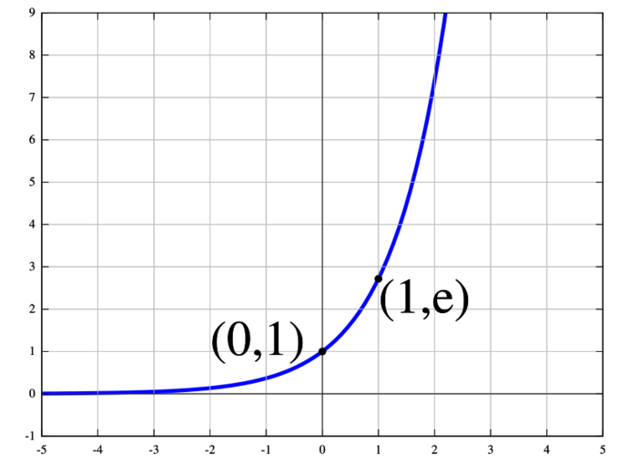
Exponential Function: The natural exponential function [latex]y = e^x[/latex].
Exponential Growth and Decay
Exponential growth occurs when the growth rate of the value of a mathematical function is proportional to the function's current value.Learning Objectives
Apply the exponential growth and decay formulas to real world examplesKey Takeaways
Key Points
- The formula for exponential growth of a variable [latex]x[/latex] at the (positive or negative) growth rate [latex]r[/latex], as time [latex]t[/latex] goes on in discrete intervals (that is, at integer times [latex]0, 1, 2, 3, \cdots[/latex]), is: [latex]x_{t} = x_{0}(1 + r^{t})[/latex] where [latex]x_0[/latex] is the value of [latex]x[/latex] at time [latex]0[/latex].
- Exponential decay occurs in the same way as exponential growth, providing the growth rate is negative.
- In the long run, exponential growth of any kind will overtake linear growth of any kind as well as any polynomial growth.
Key Terms
- exponential: any function that has an exponent as an independent variable
- linear: having the form of a line; straight
- polynomial: an expression consisting of a sum of a finite number of terms, each term being the product of a constant coefficient and one or more variables raised to a non-negative integer power
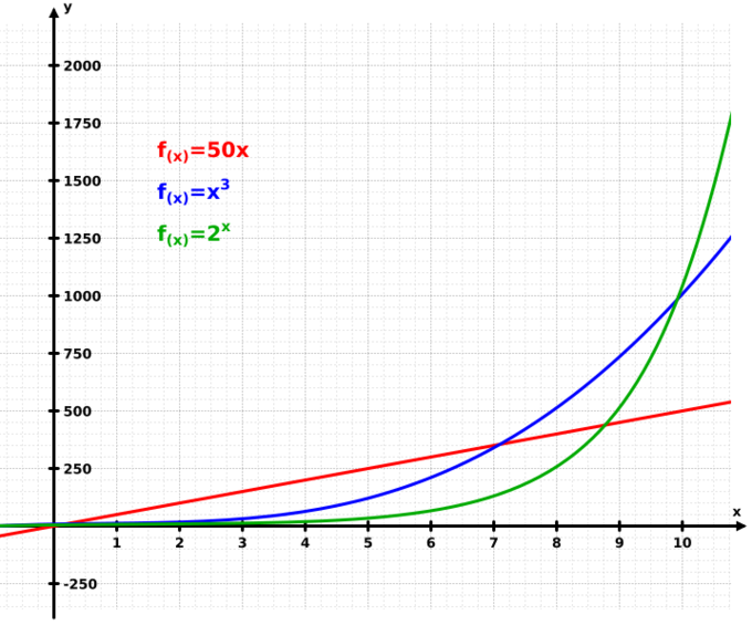
Exponential Growth: This graph illustrates how exponential growth (green) surpasses both linear (red) and cubic (blue) growth.
Inverse Trigonometric Functions: Differentiation and Integration
It is useful to know the derivatives and antiderivatives of the inverse trigonometric functions.Learning Objectives
Practice integrating and differentiating inverse trigonometric functionsKey Takeaways
Key Points
- The inverse trigonometric functions "undo" the trigonometric functions [latex]\sin[/latex], [latex]\cos[/latex], and [latex]\tan[/latex].
- The inverse trigonometric functions are [latex]\arcsin[/latex], [latex]\arccos[/latex], and [latex]\arctan[/latex].
- Memorizing their derivatives and antiderivatives can be useful.
Key Terms
- trigonometric: relating to the functions used in trigonometry: [latex]\sin[/latex], [latex]\cos[/latex], [latex]\tan[/latex], [latex]\csc[/latex], [latex]\cot[/latex], [latex]\sec[/latex]
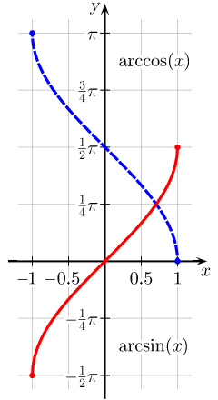
Arcsine and Arccosine: The usual principal values of the [latex]\arcsin(x)[/latex] and [latex]\arccos(x)[/latex] functions graphed on the Cartesian plane.
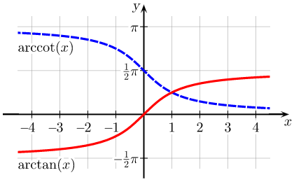
Arctangent and Arccotangent: The usual principal values of the [latex]\text{arctan}(x)[/latex] and [latex]\text{arccot}(x)[/latex] functions graphed on the Cartesian plane.
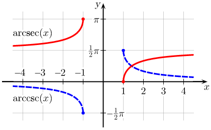
Arcsecant and Arccosecant: Principal values of the [latex]\text{arcsec}(x)[/latex] and [latex]\text{arccsc}(x)[/latex] functions graphed on the Cartesian plane.
Hyperbolic Functions
[latex]\sinh[/latex] and [latex]\cosh[/latex] are basic hyperbolic functions; [latex]\sinh[/latex] is defined as the following: [latex]\sinh (x) = \frac{e^x - e^{-x}}{2}[/latex].Learning Objectives
Discuss the basic properties of hyperbolic functionsKey Takeaways
Key Points
- The basic hyperbolic functions are the hyperbolic sine "[latex]\sinh[/latex]," and the hyperbolic cosine "[latex]\cosh[/latex]," from which are derived the hyperbolic tangent "[latex]\tanh[/latex]," and so on, corresponding to the derived trigonometric functions.
- The inverse hyperbolic functions are the area hyperbolic sine "[latex]\text{arsinh}[/latex]" (also called "[latex]\text{asinh}[/latex]" or sometimes "[latex]\text{arcsinh}[/latex]") and so on.
- The hyperbolic functions take real values for a real argument called a hyperbolic angle. The size of a hyperbolic angle is the area of its hyperbolic sector.
Key Terms
- meromorphic: relating to or being a function of a complex variable that is analytic everywhere in a region except for singularities at each of which infinity is the limit and each of which is contained in a neighborhood where the function is analytic except for the singular point itself
- inverse: a function that undoes another function
Hyperbolic sine
[latex-display]\sinh (x) = \dfrac{e^x - e^{-x}}{2}[/latex-display]Hyperbolic cosine
[latex-display]\cosh (x) =\dfrac{e^x + e^{-x}}{2}[/latex-display]Hyperbolic tangent
[latex-display]\tanh (x) = \dfrac{\sinh(x)}{\cosh (x)} = \dfrac{1 - e^{-2x}}{1 + e^{-2x}}[/latex-display]Hyperbolic cotangent
[latex-display]\coth (x) = \dfrac{\cosh (x)}{\sinh (x)} = \dfrac{1 + e^{-2x}}{1 - e^{-2x}}[/latex-display]Hyperbolic secant
[latex-display]\text{sech} (x) = (\cosh (x))^{-1}= \dfrac{2}{e^x + e^{-x}}[/latex-display]Hyperbolic cosecant
[latex-display]\text{csch} (x)= (\sinh (x))^{-1}= \dfrac{2}{e^x - e^{-x}}[/latex-display]Indeterminate Forms and L'Hôpital's Rule
Indeterminate forms like [latex]\frac{0}{0}[/latex] have no definite value; however, when a limit is indeterminate, l'Hôpital's rule can often be used to evaluate it.Learning Objectives
Use L'Hopital's Rule to evaluate limits involving indeterminate formsKey Takeaways
Key Points
- Indeterminate forms include [latex]0^0[/latex], [latex]\frac{0}{0}[/latex], [latex]1^\infty[/latex], [latex]\infty - \infty[/latex], [latex]\frac{\infty}{\infty}[/latex], [latex]0 \times \infty[/latex], and [latex]\infty^0[/latex]
- Indeterminate forms often arise when you are asked to take the limit of a function. For example: [latex]\lim_{x\to 0}\frac{x}{x}[/latex] is indeterminate, giving [latex]\frac{0}{0}[/latex].
- L'Hôpital's rule: For [latex]f[/latex] and [latex]g[/latex] which are differentiable, if [latex]\lim_{x\to c}f(x)=\lim_{x \to c}g(x) = 0[/latex] or [latex]\pm \infty[/latex] and [latex]\lim_{x\to c}\frac{f'(x)}{g'(x)}[/latex] exists, and [latex]g'(x) \neq 0[/latex] for all [latex]x[/latex] in the interval containing [latex]c[/latex], then [latex]\lim_{x \to c}\frac{f(x)}{g(x)} = \lim_{x\to c}\frac{f'(x)}{g'(x)}[/latex].
Key Terms
- limit: a value to which a sequence or function converges
- differentiable: a function that has a defined derivative (slope) at each point
- indeterminate: not accurately determined or determinable
L'Hôpital's Rule
In calculus, l'Hôpital's rule uses derivatives to help evaluate limits involving indeterminate forms. Application (or repeated application) of the rule often converts an indeterminate form to a determinate form, allowing easy evaluation of the limit. In its simplest form, l'Hôpital's rule states that for functions [latex]f[/latex] and [latex]g[/latex] which are differentiable, if [latex-display]\displaystyle{\lim_{x\to c}f(x)=\lim_{x \to c}g(x) = 0 \text{ or } \pm \infty}[/latex-display] and [latex]\lim_{x\to c}\frac{f'(x)}{g'(x)}[/latex] exists, and [latex]g'(x) \neq 0[/latex] for all [latex]x[/latex] in the interval containing [latex]c[/latex], then: [latex-display]\displaystyle{\lim_{x \to c}\frac{f(x)}{g(x)} = \lim_{x\to c}\frac{f'(x)}{g'(x)}}[/latex-display]Bases Other than e and their Applications
Among all choices for the base [latex]b[/latex], particularly common values for logarithms are [latex]e[/latex], [latex]2[/latex], and [latex]10[/latex].Learning Objectives
Distinguish between the different applications for logarithms in various basesKey Takeaways
Key Points
- The major advantage of common logarithms (logarithms to base ten) is that they are easy to use for manual calculations in the decimal number system.
- The binary logarithm is often used in computer science and information theory because it is closely connected to the binary numeral system.
- Common logarithm is frequently written as "[latex]\log(x)[/latex]"; binary logarithm is frequently written "[latex]\text{ld}\, n[/latex]" or "[latex]\lg n[/latex]".
Key Terms
- logarithm: the exponent by which another fixed value, the base, must be raised to produce that number
Licenses & Attributions
CC licensed content, Shared previously
- Curation and Revision. Provided by: Boundless.com License: CC BY-SA: Attribution-ShareAlike.
CC licensed content, Specific attribution
- Inverse function. Provided by: Wikipedia Located at: https://en.wikipedia.org/wiki/Inverse_function. License: CC BY-SA: Attribution-ShareAlike.
- inverse. Provided by: Wiktionary License: CC BY-SA: Attribution-ShareAlike.
- function. Provided by: Wiktionary License: CC BY-SA: Attribution-ShareAlike.
- Provided by: Wikimedia Located at: https://upload.wikimedia.org/wikipedia/commons/9/9d/Inverse_Functions_Domain_and_Range.png. License: CC BY-SA: Attribution-ShareAlike.
- Provided by: Wikimedia Located at: https://upload.wikimedia.org/wikipedia/commons/c/c8/Inverse_Function.png. License: CC BY-SA: Attribution-ShareAlike.
- Exponential function. Provided by: Wikipedia License: CC BY-SA: Attribution-ShareAlike.
- exponential. Provided by: Wiktionary License: CC BY-SA: Attribution-ShareAlike.
- tangent. Provided by: Wiktionary License: CC BY-SA: Attribution-ShareAlike.
- e. Provided by: Wiktionary License: CC BY-SA: Attribution-ShareAlike.
- Provided by: Wikimedia License: CC BY-SA: Attribution-ShareAlike.
- Provided by: Wikimedia License: CC BY-SA: Attribution-ShareAlike.
- Provided by: Wikimedia License: CC BY-SA: Attribution-ShareAlike.
- Logarithmic function. Provided by: Wikipedia License: CC BY-SA: Attribution-ShareAlike.
- Logarithmic function. Provided by: Wikipedia License: CC BY-SA: Attribution-ShareAlike.
- exponent. Provided by: Wiktionary License: CC BY-SA: Attribution-ShareAlike.
- binary. Provided by: Wiktionary License: CC BY-SA: Attribution-ShareAlike.
- Provided by: Wikimedia License: CC BY-SA: Attribution-ShareAlike.
- Provided by: Wikimedia License: CC BY-SA: Attribution-ShareAlike.
- Provided by: Wikimedia License: CC BY-SA: Attribution-ShareAlike.
- Binary_logarithm_plot_with_ticks.png. Provided by: Wikipedia License: CC BY-SA: Attribution-ShareAlike.
- Calculus/Derivatives of Exponential and Logarithm Functions. Provided by: Wikibooks License: CC BY-SA: Attribution-ShareAlike.
- Logarithmic functions. Provided by: Wikipedia License: CC BY-SA: Attribution-ShareAlike.
- logarithm. Provided by: Wikipedia License: CC BY-SA: Attribution-ShareAlike.
- e. Provided by: Wiktionary License: CC BY-SA: Attribution-ShareAlike.
- Provided by: Wikimedia License: CC BY-SA: Attribution-ShareAlike.
- Provided by: Wikimedia License: CC BY-SA: Attribution-ShareAlike.
- Provided by: Wikimedia License: CC BY-SA: Attribution-ShareAlike.
- Binary_logarithm_plot_with_ticks.png. Provided by: Wikipedia License: CC BY-SA: Attribution-ShareAlike.
- Natural logarithm. Provided by: Wikipedia License: CC BY-SA: Attribution-ShareAlike.
- Natural logarithm. Provided by: Wikipedia License: CC BY-SA: Attribution-ShareAlike.
- Natural logarithm. Provided by: Wikipedia License: CC BY-SA: Attribution-ShareAlike.
- transcendental. Provided by: Wiktionary License: CC BY-SA: Attribution-ShareAlike.
- irrational. Provided by: Wiktionary Located at: https://en.wiktionary.org/wiki/irrational. License: CC BY-SA: Attribution-ShareAlike.
- Provided by: Wikimedia License: CC BY-SA: Attribution-ShareAlike.
- Provided by: Wikimedia License: CC BY-SA: Attribution-ShareAlike.
- Provided by: Wikimedia License: CC BY-SA: Attribution-ShareAlike.
- Binary_logarithm_plot_with_ticks.png. Provided by: Wikipedia License: CC BY-SA: Attribution-ShareAlike.
- LogTay.png. Provided by: Wikipedia License: CC BY-SA: Attribution-ShareAlike.
- Calculus/Derivatives of Exponential and Logarithm Functions. Provided by: Wikibooks License: CC BY-SA: Attribution-ShareAlike.
- Boundless. Provided by: Boundless Learning License: CC BY-SA: Attribution-ShareAlike.
- e. Provided by: Wiktionary License: CC BY-SA: Attribution-ShareAlike.
- Provided by: Wikimedia License: CC BY-SA: Attribution-ShareAlike.
- Provided by: Wikimedia License: CC BY-SA: Attribution-ShareAlike.
- Provided by: Wikimedia License: CC BY-SA: Attribution-ShareAlike.
- Binary_logarithm_plot_with_ticks.png. Provided by: Wikipedia Located at: https://en.wikipedia.org/wiki/Logarithm. License: CC BY-SA: Attribution-ShareAlike.
- LogTay.png. Provided by: Wikipedia License: CC BY-SA: Attribution-ShareAlike.
- Exp.png. Provided by: Wikipedia License: CC BY-SA: Attribution-ShareAlike.
- Exponential growth. Provided by: Wikipedia License: CC BY-SA: Attribution-ShareAlike.
- Exponential growth. Provided by: Wikipedia License: CC BY-SA: Attribution-ShareAlike.
- polynomial. Provided by: Wiktionary License: CC BY-SA: Attribution-ShareAlike.
- linear. Provided by: Wiktionary License: CC BY-SA: Attribution-ShareAlike.
- exponential. Provided by: Wiktionary License: CC BY-SA: Attribution-ShareAlike.
- Provided by: Wikimedia License: CC BY-SA: Attribution-ShareAlike.
- Provided by: Wikimedia License: CC BY-SA: Attribution-ShareAlike.
- Provided by: Wikimedia License: CC BY-SA: Attribution-ShareAlike.
- Binary_logarithm_plot_with_ticks.png. Provided by: Wikipedia License: CC BY-SA: Attribution-ShareAlike.
- LogTay.png. Provided by: Wikipedia License: CC BY-SA: Attribution-ShareAlike.
- Exp.png. Provided by: Wikipedia License: CC BY-SA: Attribution-ShareAlike.
- Exponential.png. Provided by: Wikipedia License: CC BY-SA: Attribution-ShareAlike.
- List of integrals of inverse trigonometric functions. Provided by: Wikipedia License: CC BY-SA: Attribution-ShareAlike.
- Inverse trigonometric functions. Provided by: Wikipedia License: CC BY-SA: Attribution-ShareAlike.
- Differentiation of trigonometric functions. Provided by: Wikipedia License: CC BY-SA: Attribution-ShareAlike.
- trigonometric. Provided by: Wiktionary License: CC BY-SA: Attribution-ShareAlike.
- Provided by: Wikimedia License: CC BY-SA: Attribution-ShareAlike.
- Provided by: Wikimedia License: CC BY-SA: Attribution-ShareAlike.
- Provided by: Wikimedia License: CC BY-SA: Attribution-ShareAlike.
- Binary_logarithm_plot_with_ticks.png. Provided by: Wikipedia License: CC BY-SA: Attribution-ShareAlike.
- LogTay.png. Provided by: Wikipedia License: CC BY-SA: Attribution-ShareAlike.
- Exp.png. Provided by: Wikipedia License: CC BY-SA: Attribution-ShareAlike.
- Exponential.png. Provided by: Wikipedia License: CC BY-SA: Attribution-ShareAlike.
- Arctangent_Arccotangent.svg. Provided by: Wikipedia License: CC BY-SA: Attribution-ShareAlike.
- Arcsecant_Arccosecant.svg. Provided by: Wikipedia License: CC BY-SA: Attribution-ShareAlike.
- Arcsine_Arccosine.svg. Provided by: Wikipedia License: CC BY-SA: Attribution-ShareAlike.
- Hyperbolic function. Provided by: Wikipedia License: CC BY-SA: Attribution-ShareAlike.
- meromorphic. Provided by: Wiktionary License: CC BY-SA: Attribution-ShareAlike.
- inverse. Provided by: Wiktionary License: CC BY-SA: Attribution-ShareAlike.
- Provided by: Wikimedia License: CC BY-SA: Attribution-ShareAlike.
- Provided by: Wikimedia License: CC BY-SA: Attribution-ShareAlike.
- Provided by: Wikimedia License: CC BY-SA: Attribution-ShareAlike.
- Binary_logarithm_plot_with_ticks.png. Provided by: Wikipedia Located at: https://en.wikipedia.org/wiki/Logarithm. License: CC BY-SA: Attribution-ShareAlike.
- LogTay.png. Provided by: Wikipedia License: CC BY-SA: Attribution-ShareAlike.
- Exp.png. Provided by: Wikipedia License: CC BY-SA: Attribution-ShareAlike.
- Exponential.png. Provided by: Wikipedia License: CC BY-SA: Attribution-ShareAlike.
- Arctangent_Arccotangent.svg. Provided by: Wikipedia License: CC BY-SA: Attribution-ShareAlike.
- Arcsecant_Arccosecant.svg. Provided by: Wikipedia License: CC BY-SA: Attribution-ShareAlike.
- Arcsine_Arccosine.svg. Provided by: Wikipedia License: CC BY-SA: Attribution-ShareAlike.
- L'Hu00f4pital's rule. Provided by: Wikipedia License: CC BY-SA: Attribution-ShareAlike.
- Indeterminate form. Provided by: Wikipedia License: CC BY-SA: Attribution-ShareAlike.
- limit. Provided by: Wiktionary License: CC BY-SA: Attribution-ShareAlike.
- indeterminate. Provided by: Wiktionary License: CC BY-SA: Attribution-ShareAlike.
- differentiable. Provided by: Wiktionary License: CC BY-SA: Attribution-ShareAlike.
- Provided by: Wikimedia License: CC BY-SA: Attribution-ShareAlike.
- Provided by: Wikimedia License: CC BY-SA: Attribution-ShareAlike.
- Provided by: Wikimedia License: CC BY-SA: Attribution-ShareAlike.
- Binary_logarithm_plot_with_ticks.png. Provided by: Wikipedia License: CC BY-SA: Attribution-ShareAlike.
- LogTay.png. Provided by: Wikipedia License: CC BY-SA: Attribution-ShareAlike.
- Exp.png. Provided by: Wikipedia License: CC BY-SA: Attribution-ShareAlike.
- Exponential.png. Provided by: Wikipedia License: CC BY-SA: Attribution-ShareAlike.
- Arctangent_Arccotangent.svg. Provided by: Wikipedia License: CC BY-SA: Attribution-ShareAlike.
- Arcsecant_Arccosecant.svg. Provided by: Wikipedia License: CC BY-SA: Attribution-ShareAlike.
- Arcsine_Arccosine.svg. Provided by: Wikipedia License: CC BY-SA: Attribution-ShareAlike.
- Binary logarithm. Provided by: Wikipedia License: CC BY-SA: Attribution-ShareAlike.
- Logarithm. Provided by: Wikipedia License: CC BY-SA: Attribution-ShareAlike.
- logarithm. Provided by: Wikipedia License: CC BY-SA: Attribution-ShareAlike.
- Provided by: Wikimedia License: CC BY-SA: Attribution-ShareAlike.
- Provided by: Wikimedia License: CC BY-SA: Attribution-ShareAlike.
- Provided by: Wikimedia License: CC BY-SA: Attribution-ShareAlike.
- Binary_logarithm_plot_with_ticks.png. Provided by: Wikipedia License: CC BY-SA: Attribution-ShareAlike.
- LogTay.png. Provided by: Wikipedia License: CC BY-SA: Attribution-ShareAlike.
- Exp.png. Provided by: Wikipedia License: CC BY-SA: Attribution-ShareAlike.
- Exponential.png. Provided by: Wikipedia License: CC BY-SA: Attribution-ShareAlike.
- Arctangent_Arccotangent.svg. Provided by: Wikipedia License: CC BY-SA: Attribution-ShareAlike.
- Arcsecant_Arccosecant.svg. Provided by: Wikipedia License: CC BY-SA: Attribution-ShareAlike.
- Arcsine_Arccosine.svg. Provided by: Wikipedia License: CC BY-SA: Attribution-ShareAlike.
