Logarithms and Logistic Growth
In a confined environment the growth rate of a population may not remain constant. In a lake, for example, there is some maximum sustainable population of fish, also called a carrying capacity. In this section, we will develop a model that contains a carrying capacity term, and use it to predict growth under constraints. Because resources are typically limited in systems, these types of models are much more common than linear or geometric growth. The famous Mandelbrot set, a fractal whose growth is constrained.
Learning Objectives
- Evaluate and rewrite logarithms using the properties of logarithms
- Use the properties of logarithms to solve exponential models for time
- Identify the carrying capacity in a logistic growth model
- Use a logistic growth model to predict growth
Solve Exponentials for Time: Logarithms
Reversing an Exponent
Earlier, we found that since Olympia, WA had a population of 245 thousand in 2008 and had been growing at 3% per year, the population could be modeled by the equationPn = (1+0.03)n (245,000), or equivalently, Pn = 245,000(1.03)n.
Using this equation, we were able to predict the population in the future. Suppose we wanted to know when the population of Olympia would reach 400 thousand. Since we are looking for the year n when the population will be 400 thousand, we would need to solve the equation
400,000 = 245,000(1.03)n
Dividing both sides by 245,000 gives
1.6327 = 1.03n
One approach to this problem would be to create a table of values, or to use technology to draw a graph to estimate the solution.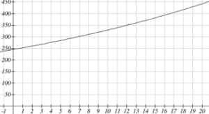 From the graph, we can estimate that the solution will be around 16 to 17 years after 2008 (2024 to 2025). This is pretty good, but we’d really like to have an algebraic tool to answer this question. To do that, we need to introduce a new function that will undo exponentials, similar to how a square root undoes a square. For exponentials, the function we need is called a logarithm. It is the inverse of the exponential, meaning it undoes the exponential. While there is a whole family of logarithms with different bases, we will focus on the common log, which is based on the exponential 10x.
Common Logarithm
Example
- log(100)
- log(1000)
- log(10000)
- log(1/100)
- log(1)
Answer:
- log(100) can be written as log(102). Since the log undoes the exponential, log(102) = 2
- log(1000) = log(103) = 3
- log(10000) = log(104) = 4
- Recall that [latex]{{x}^{-n}}=\frac{1}{{{x}^{n}}}[/latex]. [latex]\log\left(\frac{1}{100}\right)=\log\left({{10}^{-2}}\right)=-2[/latex]
- Recall that x0 = 1. log(1) = log(100) = 0
Solving exponential equations with logarithms
- Isolate the exponential. In other words, get it by itself on one side of the equation. This usually involves dividing by a number multiplying it.
- Take the log of both sides of the equation.
- Use the exponent property of logs to rewrite the exponential with the variable exponent multiplying the logarithm.
- Divide as needed to solve for the variable.
Example
If Olympia is growing according to the equation, Pn = 245(1.03)n, where n is years after 2008, and the population is measured in thousands. Find when the population will be 400 thousand.Answer: We need to solve the equation
400 = 245(1.03)n Begin by dividing both sides by 245 to isolate the exponential
1.633 = 1.03n Now take the log of both sides
log(1.633) = log(1.03n) Use the exponent property of logs on the right side
log(1.633)= n log(1.03) Now we can divide by log(1.03)
[latex]\frac{\log(1.633)}{\log(1.03)}=n[/latex] We can approximate this value on a calculator
n ≈ 16.591
A full walkthrough of this problem is available here. https://youtu.be/liNffAACIUsTry It Now
TIP
When you are solving growth problems, use the language in the question to determine whether you are solving for time, future value, present value or growth rate. Questions that uses words like "when", "what year", or "how long" are asking you to solve for time and you will need to use logarithms to solve them because the time variable in growth problems is in the exponent.Logistic Growth
Limits on Exponential Growth
In our basic exponential growth scenario, we had a recursive equation of the formPn = Pn-1 + r Pn-1
In a confined environment, however, the growth rate may not remain constant. In a lake, for example, there is some maximum sustainable population of fish, also called a carrying capacity.Carrying Capacity
The carrying capacity, or maximum sustainable population, is the largest population that an environment can support. For our fish, the carrying capacity is the largest population that the resources in the lake can sustain. If the population in the lake is far below the carrying capacity, then we would expect the population to grow essentially exponentially. However, as the population approaches the carrying capacity, there will be a scarcity of food and space available, and the growth rate will decrease. If the population exceeds the carrying capacity, there won’t be enough resources to sustain all the fish and there will be a negative growth rate, causing the population to decrease back to the carrying capacity.
If the carrying capacity was 5000, the growth rate might vary something like that in the graph shown.
For our fish, the carrying capacity is the largest population that the resources in the lake can sustain. If the population in the lake is far below the carrying capacity, then we would expect the population to grow essentially exponentially. However, as the population approaches the carrying capacity, there will be a scarcity of food and space available, and the growth rate will decrease. If the population exceeds the carrying capacity, there won’t be enough resources to sustain all the fish and there will be a negative growth rate, causing the population to decrease back to the carrying capacity.
If the carrying capacity was 5000, the growth rate might vary something like that in the graph shown.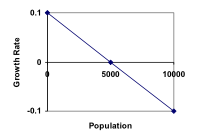 Note that this is a linear equation with intercept at 0.1 and slope [latex]-\frac{0.1}{5000}[/latex], so we could write an equation for this adjusted growth rate as:
radjusted = [latex]0.1-\frac{0.1}{5000}P=0.1\left(1-\frac{P}{5000}\right)[/latex]
Substituting this in to our original exponential growth model for r gives[latex]{{P}_{n}}={{P}_{n-1}}+0.1\left(1-\frac{{{P}_{n-1}}}{5000}\right){{P}_{n-1}}[/latex]
View the following for a detailed explanation of the concept.
https://youtu.be/-6VLXCTkP_cLogistic Growth
If a population is growing in a constrained environment with carrying capacity K, and absent constraint would grow exponentially with growth rate r, then the population behavior can be described by the logistic growth model: [latex-display]{{P}_{n}}={{P}_{n-1}}+r\left(1-\frac{{{P}_{n-1}}}{K}\right){{P}_{n-1}}[/latex-display]Examples
A forest is currently home to a population of 200 rabbits. The forest is estimated to be able to sustain a population of 2000 rabbits. Absent any restrictions, the rabbits would grow by 50% per year. Predict the future population using the logistic growth model.Answer: Modeling this with a logistic growth model, r = 0.50, K = 2000, and P0 = 200. Calculating the next year:
[latex]{{P}_{1}}={{P}_{0}}+0.50\left(1-\frac{{{P}_{0}}}{2000}\right){{P}_{0}}=200+0.50\left(1-\frac{200}{2000}\right)200=290[/latex]
We can use this to calculate the following year:[latex]{{P}_{2}}={{P}_{1}}+0.50\left(1-\frac{{{P}_{1}}}{2000}\right){{P}_{1}}=290+0.50\left(1-\frac{290}{2000}\right)290\approx414[/latex]
A calculator was used to compute several more values:| n | 0 | 1 | 2 | 3 | 4 | 5 | 6 | 7 | 8 | 9 | 10 |
| Pn | 200 | 290 | 414 | 578 | 784 | 1022 | 1272 | 1503 | 1690 | 1821 | 1902 |
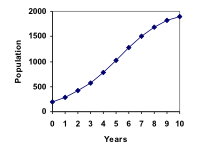 View more about this example below.
https://youtu.be/dPOlEgJ2QX0
View more about this example below.
https://youtu.be/dPOlEgJ2QX0
On an island that can support a population of 1000 lizards, there is currently a population of 600. These lizards have a lot of offspring and not a lot of natural predators, so have very high growth rate, around 150%. Calculating out the next couple generations:
[latex]{{P}_{1}}={{P}_{0}}+1.50\left(1-\frac{{{P}_{0}}}{1000}\right){{P}_{0}}=600+1.50\left(1-\frac{600}{1000}\right)600=960[/latex]
[latex]{{P}_{2}}={{P}_{1}}+1.50\left(1-\frac{{{P}_{1}}}{1000}\right){{P}_{1}}=960+1.50\left(1-\frac{960}{1000}\right)960=1018[/latex]
Interestingly, even though the factor that limits the growth rate slowed the growth a lot, the population still overshot the carrying capacity. We would expect the population to decline the next year.[latex]{{P}_{3}}={{P}_{2}}+1.50\left(1-\frac{{{P}_{3}}}{1000}\right){{P}_{3}}=1018+1.50\left(1-\frac{1018}{1000}\right)1018=991[/latex]
Calculating out a few more years and plotting the results, we see the population wavers above and below the carrying capacity, but eventually settles down, leaving a steady population near the carrying capacity.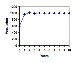
Try It Now
A field currently contains 20 mint plants. Absent constraints, the number of plants would increase by 70% each year, but the field can only support a maximum population of 300 plants. Use the logistic model to predict the population in the next three years.Answer: [latex]P_1=P_0+0.70(1-\frac{P_0}{300})P_0=20+0.70(1-\frac{20}{300})20=33[/latex] [latex-display]P_2=54[/latex-display] [latex-display]P_3=85[/latex-display]
Licenses & Attributions
CC licensed content, Original
- Introduction and Learning Objectives. Provided by: Lumen Learning License: CC BY: Attribution.
- Revision and Adaptation. Provided by: Lumen Learning License: CC BY: Attribution.
CC licensed content, Shared previously
- Math in Society. Authored by: David Lippman. Located at: http://www.opentextbookstore.com/mathinsociety/. License: CC BY-SA: Attribution-ShareAlike.
- population-statistics-human. Authored by: geralt. License: CC BY: Attribution.
- Using logs to solve for time. Authored by: OCLPhase2's channel. License: CC BY: Attribution.
- Using logs to solve an exponential. Authored by: OCLPhase2's channel. License: CC BY: Attribution.
- Question ID 100163. Authored by: Rieman, Rick. License: CC BY: Attribution. License terms: IMathAS Community License CC-BY + GPL.
- Question ID 1764. Authored by: Lippman, David. License: CC BY: Attribution. License terms: IMathAS Community License CC-BY + GPL.
- Question ID 34625. Authored by: Smart, Jim. License: CC BY: Attribution. License terms: IMathAS Community License CC-BY + GPL.
- fishes-colourful-beautiful-koi. Authored by: sharonang. License: CC0: No Rights Reserved.
- Logistic model. Authored by: OCLPhase2's channel. License: CC BY: Attribution.
- Logistic growth of rabbits. Authored by: OCLPhase2's channel. License: CC BY: Attribution.
- Logistic growth of lizards. Authored by: OCLPhase2's channel. License: CC BY: Attribution.
- Question ID 54627. Authored by: Hartley, Josiah. License: CC BY: Attribution. License terms: IMathAS Community License CC-BY + GPL.
- Question ID 6589. Authored by: Lippman, David. License: CC BY: Attribution. License terms: IMathAS Community License CC-BY + GPL.
